Yes—radar-based human activity recognition can run on an edge device, including processors integrated into a radar sensor. Feasibility depends on the complete sensing pipeline: how much motion the system must observe, how often it updates a prediction, how much working memory it needs, and how much energy it consumes while sensing and processing. A small model or a fast inference result answers only part of that question.
For a useful deployment decision, budget four things together: recognition quality, response time, peak memory and average system power. This guide explains how to measure them, uses published on-device radar evidence, and provides an original worked budget with a runnable calculator.
What published radar deployments actually demonstrate
Yadav and colleagues’ tinyRadar for Fitness implemented radar processing and an 8-bit CNN on the TI IWR1843. It classified eight exercise categories, training on ten people and reporting 97% classification accuracy on four additional people. The paper reports the following implementation figures; its KB notation is retained here.
| Reported item | tinyRadar result |
|---|---|
| CNN parameters and activations | 11.36 KB combined; parameters alone were 1.46 KB |
| Velocity-column generation buffers | 560.13 KB |
| CNN processing latency | Approximately 69 ms |
| Input history | 64 frames at 70 ms per frame: approximately 4.48 s |
| Power | Approximately 1 W, reported with the radio-frequency (RF) front end |
These results apply to the reported task and test conditions. The memory figures span different processing stages and memory regions; check each region’s available capacity. Source: Sections III and VIII, and Table II.
The engineering lesson is useful beyond this study: a compact classifier can sit inside a much larger sensing workload. Its inference time, observation history and system power describe different constraints.
First decide where the edge begins
An edge system makes its operational decision near the sensor. That can mean an on-chip processor, an external microcontroller, or a nearby embedded computer. Specify where ADC conversion, radar processing, feature construction and classification run before comparing platforms.
| Architecture | Useful starting point | What to verify |
|---|---|---|
| Radar with integrated processing | A compact sensor that exports activity labels or compact features | Which processing engines and memory regions remain available after the radar firmware runs |
| Radar plus a microcontroller | A controlled task with compact features and a small model | Sensor-link throughput, shared RAM, supported operators and acquisition timing |
| Radar plus an embedded Linux board or accelerator | Larger representations, several targets or rapid prototyping | Transfers, sustained performance, operating-system delays and whole-board power |
LiteRT for Microcontrollers supports inference on small devices but has a limited operator set and requires manual memory management. Runtime compatibility therefore belongs in the first prototype, before extensive architecture tuning. Our ADC-to-label radar-HAR pipeline guide explains the processing stages that must accompany the model.
Latency: separate observation time, update interval and processing delay
“Real time” needs a deadline. A room-activity dashboard and an urgent event detector may tolerate very different delays. Record exactly when the relevant event starts and when the application emits a usable decision.
| Quantity | Meaning |
|---|---|
| Observation window | How much recent motion contributes to one prediction |
| Prediction hop | How much new time passes between successive input windows |
| Processing delay | Time from a ready input window to its output |
| Event-to-decision latency | Time from a defined physical event to the emitted decision, including the decision policy |
A two-second window can slide forward every 100 ms. After startup, that produces ten prediction opportunities per second. It does not make the first complete window available after 100 ms, and it does not guarantee that every new activity becomes recognizable within one hop.
A worked timing budget
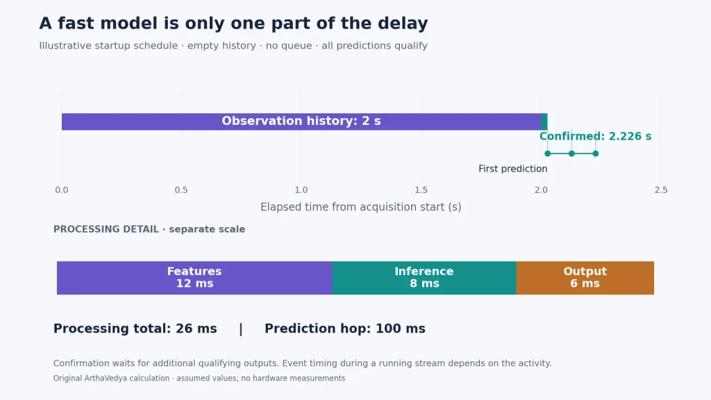
The numbers in the worked example below are illustrative assumptions, not measurements from a particular radar or processor. Assume a two-second causal input window and a 100 ms prediction hop. Once each input is ready, feature preparation takes 12 ms, inference takes 8 ms, and output handling takes 6 ms. These serial stages include the work assigned to that prediction update.
T_{\mathrm{step}}=T_{\mathrm{features}}+T_{\mathrm{inference}}+T_{\mathrm{output}}.The processing total is 26 ms per update. With an initially empty history, no queue and this processing placed after window completion, the first prediction becomes available at 2.026 s. Acquisition and feature processing may overlap in a real implementation; measure its actual schedule instead of adding overlapping durations twice.
T_{\mathrm{first}}=T_{\mathrm{observation}}+T_{\mathrm{step}}.Now require three consecutive qualifying predictions before emitting an activity change. In the favourable case where the first eligible prediction and the next two all qualify, confirmation adds two hops: 200 ms. The first confirmed output from that empty-history startup is therefore 2.226 s. This is a conditional timing example, not a bound on detecting an event during an already running stream.
Keep the pipeline causal and check every deadline
A centred time window needs samples on both sides of its timestamp. A forward-and-backward filter needs future samples or a completed segment. An offline classifier can therefore appear to recognize an event before the data needed for its features would be available online. Define whether timestamps mark the start, centre or end of the contributing interval. Our STFT parameter guide explains the underlying time–frequency trade-off.
For a simple serial update task, 26 ms of work inside a 100 ms hop leaves 74 ms before the next update. That arithmetic alone does not prove schedulability. The radar may also need frame processing every 50 ms; interrupts, transfers and other tasks may share the same processor or memory bus. Check each acquisition and processing deadline, then measure queue growth, dropped frames and the age of emitted predictions.
If processing falls behind, choose a deliberate policy. Preserving every window can produce increasingly stale outputs. Discarding old windows can preserve freshness but may miss brief events. Report that policy and evaluate its consequences on continuous recordings.
Choose the representation before shrinking the model
The representation determines which information reaches the classifier and how much data the device must move. Start with the physical cues needed to distinguish the activities, then test a compact representation that retains those cues.
| Representation | Potential saving | Question to test |
|---|---|---|
| Engineered features or tracks | Small inputs and simple classifiers | Do the selected summaries preserve the differences between your activities? |
| Velocity–time or micro-Doppler map | A compact history after reducing spatial dimensions | Does reducing range or angle mix people or remove useful separation? |
| Point-cloud sequence | Sparse input instead of a dense cube | Do detection thresholds, missing points or point-count caps remove important motion? |
| Dense map or radar-cube sequence | Rich spatial and motion information | Does its accuracy gain justify acquisition, buffering and compute costs? |
These are design trade-offs, not a universal ranking. A point cloud can be sparse at the sensor interface yet expensive after voxelization. A small spectrogram model can still depend on costly fast Fourier transforms (FFTs) and a large radar cube. Include the cost of constructing the representation in every comparison.
Memory: a model file is not the RAM budget
Separate persistent storage, such as firmware and model constants, from working RAM, such as acquisition buffers, FFT workspace, feature history, neural-network activations, stacks and communication buffers. Some systems read weights directly from flash; others copy them into RAM. Count the implementation you will actually deploy.
For example, TensorFlow Lite Micro’s memory-management documentation describes a tensor arena with reusable, temporary and persistent allocations. Buffer lifetimes matter: tensors that are never needed together may share storage. The sum of every layer’s output size is therefore not automatically the peak arena requirement. Obtain the allocation report for the compiled model and account for memory outside that arena separately.
Count complex radar samples correctly
Consider one assumed frame containing 256 samples per chirp, 128 acquired chirps and four receive channels. Store each sample as signed 16-bit in-phase (I) plus signed 16-bit quadrature (Q) components. Each complex sample then occupies four bytes; “16-bit I/Q” does not mean two bytes for the pair.
B_{\mathrm{frame}}=N_s N_c N_{\mathrm{RX}} N_{\mathrm{components}}\frac{b}{8}.Here, Ns is samples per chirp, Nc is acquired chirps per frame, NRX is receive channels, and b is bits per stored component. This example has two components. The frame payload is 524,288 bytes, or 512 KiB. Double buffering needs 1 MiB before alignment, metadata or other workspace. One KiB is 1,024 bytes; one MiB is 1,024 KiB.
At 20 frames/s, retaining two seconds of these raw frames needs 20 MiB. Streaming the same payload off the sensor requires 10 MiB/s, about 83.9 Mbit/s, before transport overhead. A packed real-ADC stream, compressed cube or different chirp schedule produces a different answer. For time-division MIMO, count the acquired chirps and actual stored channel dimensions; do not multiply by virtual antennas again without checking the layout.
Keep only the history the algorithm needs
Suppose the streaming front end reduces each frame to 64 velocity values. Forty frames then form a 64 × 40 input. That history occupies 2.5 KiB at int8, or 10 KiB at float32. A ring buffer can update it without retaining forty raw cubes, although the front end still needs its own working buffers and this reduction discards information.
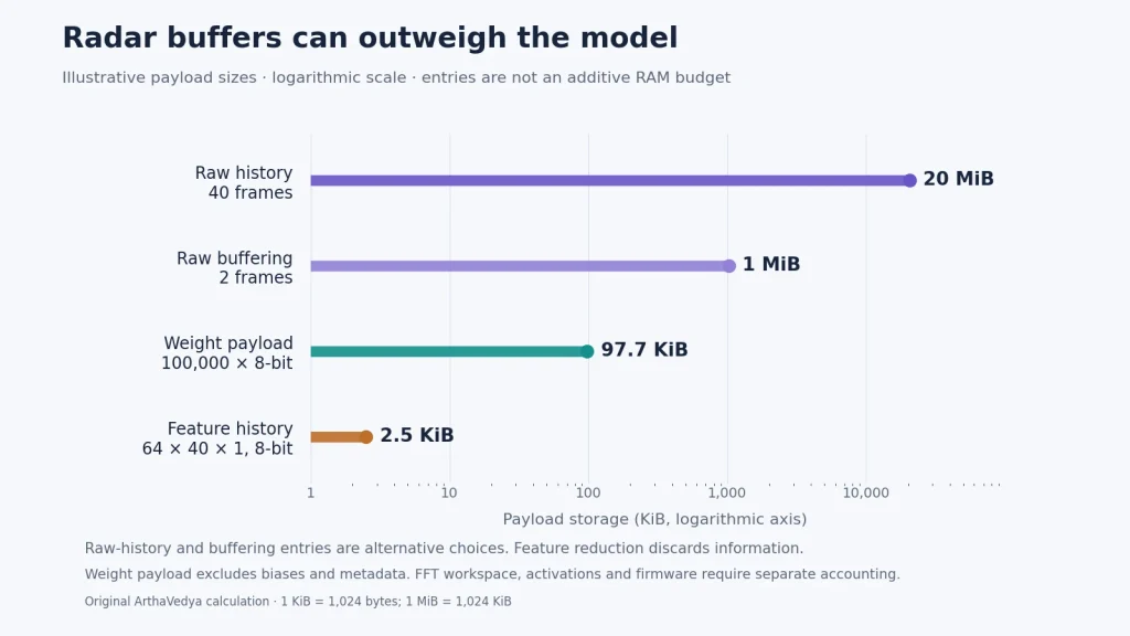
For comparison, 100,000 int8 weights occupy about 97.7 KiB, excluding biases and metadata. Even one 32 × 40 × 16 int8 activation tensor occupies 20 KiB. Neither number establishes the full model arena size. Check simultaneous live allocations, scratch requirements, memory-bank access and firmware reservations before declaring that the system fits.
Quantization: verify the exported graph and the recognition quality
Representing a weight with eight bits instead of 32 gives a fourfold reduction in its raw storage. It does not guarantee fourfold lower RAM, latency or power. The LiteRT 8-bit specification uses scales and zero points, and convolution biases can remain int32. Radar preprocessing can also continue to use wider fixed-point or floating-point arithmetic.
Google’s integer-quantization guide explains representative-data calibration and warns that a successful conversion can retain floating-point inputs, outputs or unsupported operations. For an integer-only target, request an integer-only graph and inspect the resulting operators, tensor types and accelerator assignments.
- Build calibration inputs through the same preprocessing, scaling and clipping rules used by the device. Cover representative motion strengths, ranges and backgrounds from the permitted development data.
- Keep the protected test people, sessions or rooms out of calibration unless the evaluation explicitly permits target-data access.
- Compare floating-point and deployed predictions on the same held-out recordings. Inspect per-class recall and transition behaviour, not only overall accuracy.
- If post-training quantization causes unacceptable loss, investigate saturation, scaling and unsupported operators before trying quantization-aware training or changing the architecture.
Our guide to subject leakage, splits and domain shift explains why deployment optimization must preserve the evaluation boundary. A smaller model should not receive a more favourable test protocol.
Operator implementation matters too. Arm’s CMSIS-NN documentation describes optimized kernels and processor-specific implementations for Cortex-M devices. Measure the compiled path on your target. A lower operation count can still run more slowly if it introduces inefficient shapes, extra memory movement or poorly supported operators.
Power: measure the configured system at a named boundary
State whether a power number covers the processor, radar chip, sensor module or complete device input. The RF front end, clocking, signal processing, regulators, indicator LEDs and wireless link can all contribute. A processor’s low-power specification does not describe a radar installation that continuously acquires data.
TI’s TIDA-010254 reference design demonstrates battery-powered radar with wireless communication for counting and tracking. It is useful implementation evidence, but its task is not a general radar-HAR benchmark. A low-power occupancy or tracking configuration cannot supply the power figure for an arbitrary activity-recognition pipeline.
Use average power and energy per update together
For a simplified device that alternates between two non-overlapping operating states, average power depends on both state power and time spent in each state:
P_{\mathrm{avg}}=dP_{\mathrm{active}}+(1-d)P_{\mathrm{idle}}.Here, d is the active fraction of the observation period, and both power values refer to the same measurement boundary. This operating-state fraction is not automatically the RF transmit duty cycle. A real device may require more than two states, including RF startup, acquisition, processing and transmission.
As a separate illustrative power assumption, let the entire device draw 0.60 W for 26 ms and 0.12 W for the remaining 74 ms of each 100 ms period. Its average power is 244.8 mW; energy per scheduled update is 24.48 mJ. The calculation assumes those states cover all device activity, including sensing. It is not a power prediction derived from the timing budget.
If an optimization reduces inference from 8 ms to 2 ms, and all six recovered milliseconds really move the whole device into its lower-power state, average power falls to 216.0 mW: an 11.8% reduction, despite a fourfold faster inference stage. If radar acquisition or another task prevents that state change, the saving can be smaller or absent.
Reducing frame rate or waking only after a trigger may save more energy, but it changes what the sensor observes. Test missed short activities, wake-up delay and trigger errors. Reducing chirps can also alter Doppler resolution and integration gain. Treat each sensing configuration as a new operating point that needs quality evaluation.
Measure voltage and current across a representative continuous run, with enough time resolution to capture operating bursts. Integrate power over time, include startup and radio activity where relevant, and report the workload duration. State whether the energy denominator is scheduled updates, emitted labels or detected events. Empty-room operation and continuous human motion may have different costs.
A deployment workflow that produces comparable results
Start with one modest baseline and one clearly stated task. Compile a small end-to-end prototype early so that sensor access, operator support and buffer constraints shape the design.
- Define the acceptance criteria. Specify activities, people and rooms, single- or multi-person operation, event timestamps, tolerated delay and the consequence of a false alarm.
- Freeze a sensor and preprocessing configuration. Record chirps, frame rate, antenna use, numerical formats, clutter removal, feature scaling, history length and prediction hop.
- Compare device features with a desktop reference. Replay the same recording through both implementations; inspect intermediate values before attributing output differences to the model.
- Export, allocate and profile. Record the actual model file, firmware build, operator placement, arena allocation, other live buffers and processing times.
- Run continuous held-out streams. Include empty scenes, transitions, ambiguous motion and the population the intended claim covers. Measure the complete decision policy.
- Change one constraint at a time. Test smaller inputs, quantization, shorter histories or duty cycling against the same protected evaluation protocol.
Plan coverage with our radar-HAR dataset collection guide. Window classification on carefully trimmed clips does not establish continuous monitoring performance. Report missed events and false alarms over recorded time when the application emits events, and keep the matching rule explicit.
What to put in the benchmark report
| Budget | Minimum useful report |
|---|---|
| Recognition | Split and population; class-level results; event misses and false alarms where applicable |
| Timing | Observation window and hop; processing p50/p95/p99 and observed maximum; event-to-decision distribution |
| Scheduling | Frame deadlines, queue depth, dropped-frame count and stale-output policy |
| Memory | Model and firmware storage; peak RAM by region; tensor arena, radar buffers, stacks and reserved space |
| Power | Measurement boundary; voltage, average power, energy denominator, operating mode and run duration |
| Reproducibility | Board, clocks, software versions, compiler settings, numerical formats and model identifier |
Here, p50, p95 and p99 denote the 50th, 95th and 99th percentiles. Use batch size one for a single streaming decision unless the deployed system actually batches. Warm up accelerators where needed, synchronize asynchronous work before stopping the timer, and test sustained operation after temperatures stabilize. Report cold-start behaviour separately. An observed maximum or p99 from a finite run is not a proven worst-case execution bound.
Local inference can reduce dependence on a network and avoid exporting raw radar measurements. Activity labels and stored histories can still reveal sensitive behaviour; choose retention and communication rules deliberately. Our radar-versus-camera monitoring comparison discusses that broader system decision.
Use the companion calculator as a budget worksheet
The companion Python calculator reproduces the illustrative arithmetic and both figures. It accepts a JSON configuration for raw-frame dimensions, feature history, processing times and a separate two-state power schedule. With no configuration, it uses the clearly labelled example in this article.
python radar_edge_budget.py --output-dir edge-budgetIt reports raw payload size and rate, history storage, weight payload, startup timing, conditional confirmation delay and average power. It also flags when the assumed serial update cannot finish inside its hop. Read that as a screening calculation: the tool does not execute a model, measure hardware, infer peak RAM from weights, or certify a real-time schedule.
Use measured inputs as the prototype matures. Keep separate records for assumptions and measurements, then use the benchmark report above to decide whether a candidate meets the application’s requirements.
How to decide whether your radar-HAR system belongs on the edge
A compact radar-HAR task is a strong candidate when the front end can maintain a useful representation within available memory, the complete schedule meets the response requirement, and recognition quality remains acceptable after conversion. A larger embedded computer can be appropriate when spatial detail, multiple targets or model complexity justify its resource cost.
- If response is too slow: inspect observation history, confirmation rules and queueing alongside inference time.
- If RAM is exhausted: inspect radar buffers, feature history and activation lifetimes before focusing only on parameter count.
- If power is too high: measure which operating states dominate, then verify the recognition cost of changing them.
- If quality drops: compare sensing, preprocessing and exported numerics under the same evaluation protocol.
Choose the least costly implementation that meets the stated task and the evidence required to support it. The useful result is a reproducible operating point—recognition quality, delay, memory and power measured together.
References
- Yadav, S. S., Agarwal, R., Bharath, K., Rao, S., and Thakur, C. S. (2023). tinyRadar for Fitness: A Contactless Framework for Edge Computing. Author-hosted manuscript; implementation results in Section VIII.
- Google AI Edge. LiteRT for Microcontrollers. Runtime scope, deployment workflow and limitations.
- TensorFlow Lite Micro contributors. Memory Management in TensorFlow Lite Micro. Arena allocation and buffer reuse.
- Google AI Edge. Post-training integer quantization. Calibration and integer-only conversion.
- Google AI Edge. LiteRT 8-bit quantization specification. Tensor formats and operator requirements.
- Arm. CMSIS-NN software library documentation. Optimized inference kernels.
- Texas Instruments. TIDA-010254: Battery-powered mmWave radar sensor reference design. Counting and tracking implementation context.