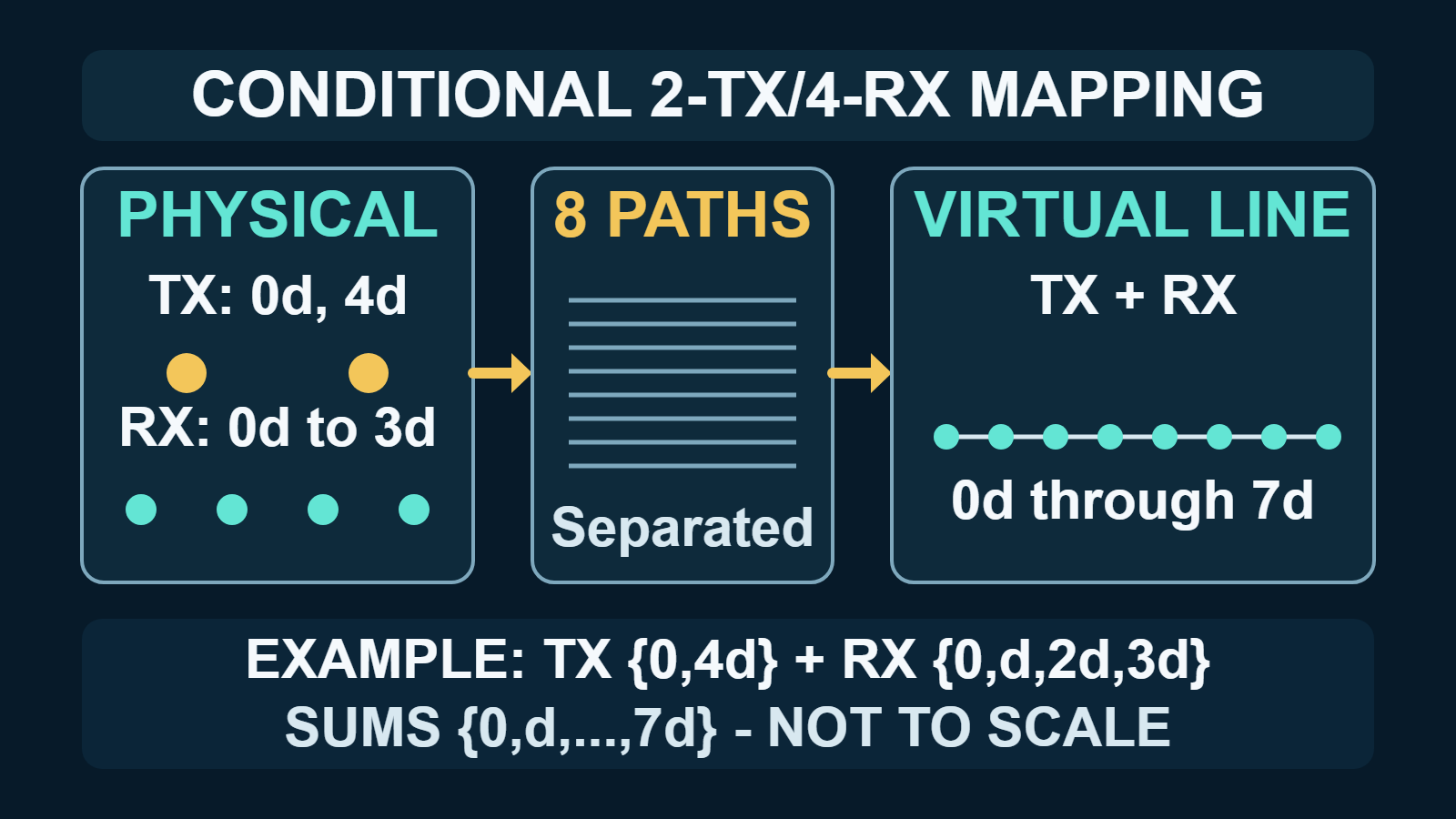
Short answer: a coherent, colocated MIMO radar does not create extra physical receivers. It separates the echo from each transmitter at every receiver, producing one complex measurement for each transmit–receive pair. Under a far-field, narrowband model, the phase of that pair is equivalent to a sample at the summed transmit and receive coordinate. If those sums form a useful, calibrated aperture, a small physical array can behave spatially like a larger virtual array.
The multiplication rule needs a qualification: MT transmitters and NR receivers produce MT × NR pair channels, but not automatically that many distinct, uniformly spaced positions. Duplicate sums, holes, channel errors, waveform leakage, and transmitter timing can all reduce or distort the usable array. The geometry must be enumerated before selecting an angle-processing model.
What “virtual array” means in this guide
This guide concerns coherent, colocated or quasi-monostatic MIMO radar: the transmit and receive apertures are close enough that a target is represented by effectively the same far-field direction at every element. Widely separated MIMO radar is a different architecture, commonly used to exploit spatial diversity in a target’s response. The distinction matters because the simple summed-coordinate construction belongs to the colocated model, as discussed in Hassanien and Vorobyov’s phased-MIMO treatment and the minimum-redundancy MIMO array study.
Three counts should be kept separate:
- Physical elements: the antennas and receiver chains that exist in hardware.
- Pair channels: the separable complex measurements indexed by transmitter and receiver.
- Distinct virtual coordinates: the unique spatial sums represented by those pair channels.
A repeated coordinate can provide another noisy observation and can change the effective weighting, but it does not extend the geometric aperture. The minimum-redundancy MIMO array study and the thinned-virtual-array study make this distinction explicit: virtual data-vector length, unique locations, aperture, sidelobes, and direction-estimation performance are related quantities, not synonyms.
The prerequisites: separability, coherence, and a valid propagation model
The construction works only when the receiver can identify which transmitter produced each contribution. Matched filtering, time slots, phase codes, or another valid demultiplexing method must recover each transmitter’s complex echo at each receiver. Texas Instruments’ MIMO Radar application report describes time-division multiplexing (TDM) and binary phase modulation (BPM) as two such strategies. They are examples, not the only possible choices.
The recovered channels must remain phase coherent. Magnitude-only data cannot preserve the spatial phase progression used for direction finding, and unknown relative channel phase can masquerade as target angle; the coherent virtual-steering model and its colocated assumptions are set out in the TI MIMO Radar application report, Hassanien and Vorobyov’s phased-MIMO treatment, and the minimum-redundancy MIMO array formulation. Finally, the elementary sum model assumes a narrowband plane wave in the far field. Near-field focusing, wideband array effects, or a genuinely bistatic layout require path-length models that cannot be replaced by the derivation below.
Why transmit and receive coordinates add
Place the transmit and receive elements along one axis. Let xT,m be the coordinate of transmitter m in metres, xR,n the coordinate of receiver n in metres, λ the wavelength in metres, θ the target direction measured from array broadside, and j the imaginary unit, so that j squared equals −1. Choose a negative complex-exponential convention and absorb range, reflectivity, and common phase into the complex amplitude α. For one far-field point target, the separated pair measurement has the spatial phase
y_{m,n}(\theta)=\alpha\exp\!\left[-j\,\frac{2\pi}{\lambda}\left(x_{\mathrm{T},m}+x_{\mathrm{R},n}\right)\sin\theta\right]The sign changes under other mixer or steering-vector conventions; the summed coordinate does not. The transmit leg contributes phase according to xT,m, the receive leg contributes phase according to xR,n, and their product adds the exponents. Pair (m,n) is therefore phase-equivalent to a one-way array sample at xT,m + xR,n. This phase-sum construction is documented in the TI MIMO Radar application report, Hassanien and Vorobyov’s steering-vector derivation, and the minimum-redundancy MIMO array formulation.
With transmitter-major stacking—all receive entries for one transmitter followed by those for the next—the MTNR-entry virtual steering vector is:
\mathbf{v}(\theta)=\mathbf{a}_{\mathrm{T}}(\theta)\otimes\mathbf{a}_{\mathrm{R}}(\theta)Here aT is the transmit steering vector, aR is the receive steering vector, and ⊗ denotes the Kronecker product. Some authors plot the midpoint (xT + xR)/2 and use a two-way wavenumber. That is a scaled coordinate convention for the same phase. Mixing the midpoint and sum conventions without rescaling is the actual error.
Worked example: two transmitters and four receivers
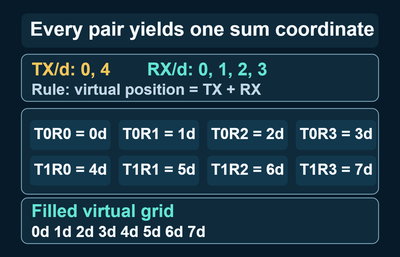
Let the receive spacing be d metres. Put four receivers at 0, d, 2d, and 3d, and put two transmitters at 0 and 4d. For the general filled-array construction, use zero-based receiver index n from 0 through NR − 1 and transmitter index m from 0 through MT − 1:
x_{\mathrm{R},n}=nd,\qquad x_{\mathrm{T},m}=mN_{\mathrm{R}}d,\qquad x_{\mathrm{V},m,n}=\left(mN_{\mathrm{R}}+n\right)dIn this example, m is 0 or 1 and n runs from 0 through 3. The first transmitter produces coordinates 0 through 3d; the second produces 4d through 7d. The eight pair channels therefore occupy eight distinct contiguous positions. This is the specific 2-TX/4-RX geometry in the TI application report—not a guarantee for every two-transmitter, four-receiver layout.
| Transmitter coordinate | With RX at 0 | With RX at d | With RX at 2d | With RX at 3d |
|---|---|---|---|---|
| 0 | 0 | d | 2d | 3d |
| 4d | 4d | 5d | 6d | 7d |
Reproduce the coordinate check
This standard-library Python example expresses distance in wavelengths, sets d to half a wavelength, and prints every pair coordinate and its multiplicity. Change the transmit or receive lists to audit another layout.
from collections import Counter
from fractions import Fraction

d = Fraction(1, 2)  # wavelength units; exact, not binary float
rx = [n * d for n in range(4)]
tx = [m * len(rx) * d for m in range(2)]

pairs = [
    (tx_index, rx_index, tx_pos + rx_pos)
    for tx_index, tx_pos in enumerate(tx)
    for rx_index, rx_pos in enumerate(rx)
]
counts = Counter(position for _, _, position in pairs)

print("TX coordinates:", tx)
print("RX coordinates:", rx)
print("Pair coordinates:", pairs)
print("Multiplicity:", sorted(counts.items()))
The result contains eight pair channels at 0, 0.5, 1.0, …, 3.5 wavelengths, each with multiplicity one. That output verifies the arithmetic only. It does not validate antenna patterns, mutual coupling, synchronization, calibration, or a real radar implementation.
Why MT × NR can be the wrong headline number
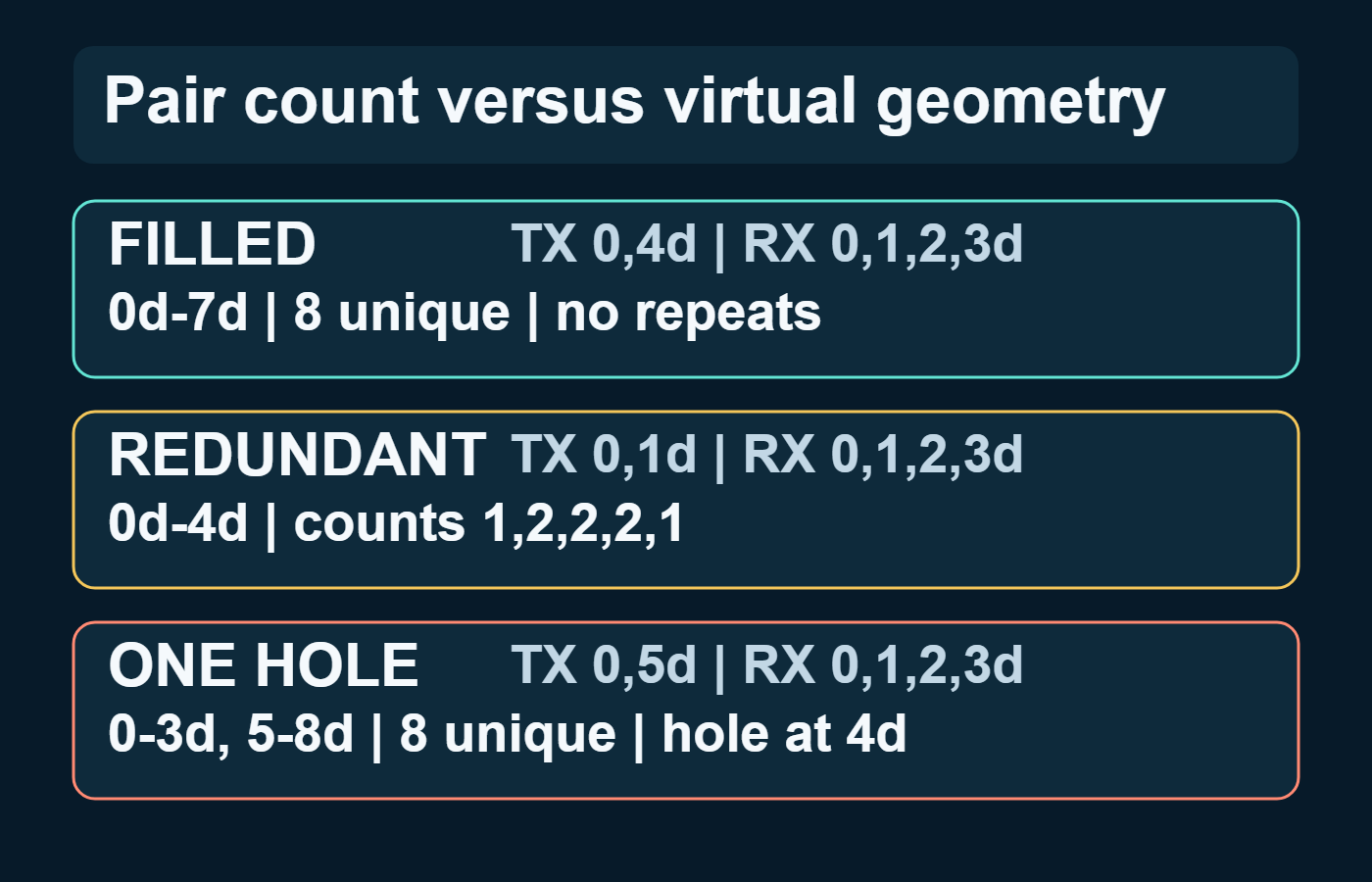
The same number of physical antennas can create very different virtual geometries. The following three layouts are calculated from the sum rule; they are geometry examples, not measured performance results.
| TX coordinates | RX coordinates | Pair channels | Unique coordinates | What changes |
|---|---|---|---|---|
| {0, 4d} | {0, d, 2d, 3d} | 8 | 8 | Filled grid from 0 to 7d |
| {0, d} | {0, d, 2d, 3d} | 8 | 5 | Repeated positions at d, 2d, and 3d; aperture ends at 4d |
| {0, 5d} | {0, d, 2d, 3d} | 8 | 8 | One missing grid point at 4d; aperture extends to 8d |
In the second layout, multiple pair channels share coordinates. Averaging properly calibrated repeated observations may help noise performance, but the duplicates do not add new baselines. In the third, the larger nominal aperture comes with a hole on an otherwise uniform spatial lattice. An FFT can still be used when the absent coordinate is represented by a zero weight, or by an equivalent explicit spatial mask, but that sparse weighting changes the array factor, sidelobes, and ambiguity. Packing the surviving channels as contiguous samples—or claiming filled-ULA performance—is invalid. The thinned-virtual-array study further shows that direction-dependent Fisher information, redundancy, aperture, ambiguity, and sidelobe behaviour all enter array design.
Angular resolution follows populated geometry, not multiplication alone
For a filled uniform linear array with N usable positions separated by d metres, conventional unwindowed FFT beamforming near broadside is often summarized by
\Delta\theta_{\mathrm{FFT}}\approx\frac{\lambda}{Nd},\qquad d=\frac{\lambda}{2}\ \Longrightarrow\ \Delta\theta_{\mathrm{FFT}}\approx\frac{2}{N}\ \mathrm{radians}The January 2026 revision of TI’s resolution brief limits this approximation to the classic case of static point targets at the same range and distinguishes angular resolution from angular accuracy. It is not a universal MIMO bound. Off-boresight geometry, tapering, sparse sampling, SNR, element patterns, mutual coupling, calibration, correlated targets, snapshots, and the estimator can all change practical results.
A larger well-populated aperture can narrow the main lobe, but simply adding a transmitter does not guarantee a fixed improvement factor. As the filled-array constructions in the TI MIMO Radar application report and Hassanien and Vorobyov’s phased-MIMO treatment show, half-wavelength spacing must be checked on the effective virtual grid and the composite transmit–receive response. A physical transmit separation larger than half a wavelength can be valid when receiver offsets interleave the sums into a filled half-wavelength virtual grid. For the role of wavelength in physical layout choices, see ArthaVedya’s guide to choosing between 24, 60, and 77 GHz radar.
How pair measurements enter an FMCW processing chain
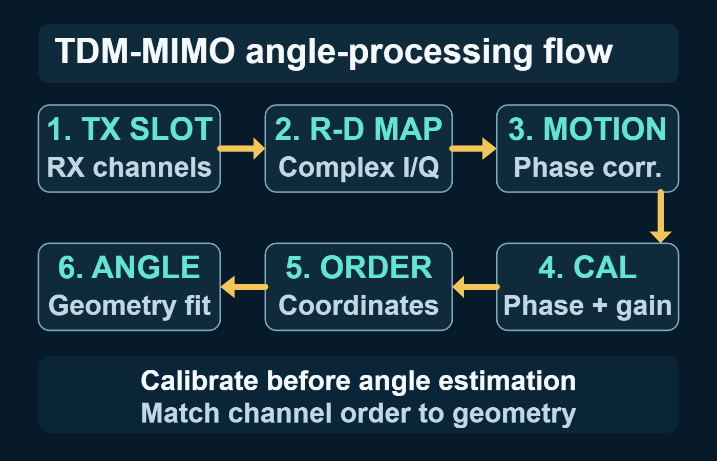
In a common TDM-FMCW implementation, transmitters take successive chirp slots. The processing examples in the TI MIMO Radar application report and TI’s cascaded imaging-radar reference design support a typical chain that forms a range–Doppler response for each transmit–receive pair, combines channel power for detection, and then performs angle processing on the calibrated complex pair values at a detected range–Doppler cell. The exact transform order, detector, and data layout remain implementation-specific. This preserves an important distinction: noncoherent power combination can support detection, but the angle estimator still needs coherent complex samples. ArthaVedya’s guide to range–Doppler–angle processing places that spatial step in the wider radar-cube workflow.
- Separate the samples by transmitter schedule and receiver.
- Compute range and Doppler responses with the correct slow-time interval for each transmitter.
- Detect candidate range–Doppler cells using an explicitly defined combination of channel power.
- Extract the complex value from every usable pair channel at each candidate cell.
- Apply relative channel calibration and the transmitter-dependent motion correction required by the schedule.
- Order samples by virtual coordinate and use an estimator that matches the populated geometry.
The TDM motion trap
TDM makes transmit contributions separable by sampling them at different times. That time offset is harmless for a stationary point target, but radial motion adds transmitter-dependent Doppler phase. If the samples are concatenated as though they were simultaneous, an angle estimator can interpret the resulting phase step as spatial phase. Bechter, Roos, and Waldschmidt derive this error and a transmitter-aware correction in their TDM-MIMO motion-compensation paper.
The correction depends on the Doppler estimate and the actual transmitter timing. A wrong aliased velocity can therefore select the wrong phase correction and turn velocity ambiguity into angle ambiguity, as documented in TI’s traffic-monitoring reference design. A single constant-Doppler correction is also only a model: acceleration, micro-Doppler, range migration, or unresolved movers with different velocities can leave residual errors. For acquisition-level ordering checks, see the TDM-MIMO trap in raw radar processing.
Relative channel calibration is part of the array
The virtual steering model presumes known relative phase and gain. RF paths, antenna placement, board routing, and frequency response violate that ideal. TI’s cascaded imaging-radar reference design estimates and applies per-pair frequency, phase, and amplitude corrections and recommends calibration for the particular board. Its target geometry and processing recipe are design-specific; they do not establish that one calibration remains sufficient across every temperature, enclosure, mounting condition, and operating frequency.
TDM, phase coding, and phased-MIMO are not interchangeable
| Approach | How transmit contributions are separated | Main point for virtual-array processing | Important qualification |
|---|---|---|---|
| TDM-MIMO | One transmitter occupies each scheduled time slot | Separate pair channels are simple to form | Sequential timing couples motion phase into the spatial vector |
| Binary phase modulation | Simultaneous transmitters use decodable phase codes | Decode transmitter contributions before stacking virtual channels | Leakage, code assumptions, power, and ambiguity depend on the implementation |
| Canonical orthogonal-waveform colocated MIMO | Receiver processing separates orthogonal transmitter waveforms | Provides the full pair-data dimension under the assumed model | The standard comparison trades conventional coherent transmit-array gain for waveform diversity |
| Phased-MIMO | Coherent transmit subarrays use orthogonal inter-subarray waveforms | Creates an intermediate virtual-data dimension | The resolution-versus-coherent-gain tradeoff depends on normalization, geometry, waveforms, and processing |
The label “MIMO” does not by itself specify which row applies. A defensible analysis states the waveform or schedule, the normalization, the physical geometry, and the receiver processing before comparing resolution, SNR, robustness, or power.
A geometry-first design and review checklist
- State the propagation regime. Record whether the model is far-field and narrowband, and whether transmit and receive arrays share one target direction.
- Declare the coordinate convention. List every physical transmit and receive coordinate in metres or wavelengths, and say whether plots use sums with a one-way wavenumber or midpoints with a two-way wavenumber.
- Enumerate all pair sums. Store the transmitter index, receiver index, coordinate, and multiplicity. Do not stop at the product of the antenna counts.
- Inspect the populated grid. Measure the aperture, spacing, repeated coordinates, and holes. Analyse ambiguity and sidelobes for sparse or irregular arrays.
- Match the estimator to the geometry. For a filled uniform grid, a simple angle FFT can use the calibrated samples directly. For a uniform lattice with holes, preserve the absent coordinates with zero insertion or explicit spatial weights and analyse the resulting sparse array factor; never pack the surviving channels as though they were contiguous. Genuinely nonuniform coordinates require geometry-aware beamforming or another validated model-based estimator.
- Preserve and calibrate complex data. Verify channel ordering, phase coherence, relative gain, failed channels, and calibration stability.
- Model the multiplexing clock. Include each transmitter’s sampling offset, Doppler ambiguity, and the limits of any motion correction.
- Test the claimed capability. Use controlled point targets at known angles and velocities, then test two-target separation, off-boresight behaviour, sidelobes, and environmental drift. Keep resolution, accuracy, identifiability, and estimator variance distinct.
Failure modes that survive a plausible-looking angle plot
- Counting pairs as unique elements: duplicate coordinate sums inflate the channel count without extending aperture.
- Applying half-wavelength spacing to the wrong array: the effective grid and composite response matter; physical transmit spacing alone can be misleading.
- Concatenating TDM channels without time correction: target Doppler becomes an artificial spatial phase step.
- Using magnitude instead of complex data: the spatial phase required for signed direction information has already been discarded.
- Treating sparse or nonuniform geometry as a filled ULA: a uniform lattice with holes can use an FFT only when the missing coordinates remain explicit zero weights; the sparse mask changes sidelobes and ambiguity. Genuinely nonuniform coordinates require their actual steering geometry.
- Treating phase equivalence as hardware equivalence: a virtual eight-position sequence is not identical to eight simultaneous receiver chains in noise, coupling, dynamic range, transmit power, timing, or calibration burden.
- Inferring detection gain from virtual count: no universal SNR, range, or detection-probability improvement follows from pair count alone.
What this model does not establish
The derivation explains far-field spatial sampling; it is not a link budget, a measured benchmark, a near-field imaging model, or a purchasing recommendation. It omits element-pattern variation, mutual coupling, waveform cross-correlation, synchronization error, RF nonlinearity, multipath, extended targets, and temperature-dependent drift. It also does not prove that the largest nominal aperture is best: sparse holes can increase ambiguity and sidelobes, while Fisher information can vary with direction.
Different physical layouts can realize the same sum coordinates, and the TI MIMO Radar application report documents that the construction extends to two dimensions. Even then, azimuth and elevation can have different apertures, redundancy, and failure modes. A two-dimensional antenna drawing is useful only after its virtual baselines are enumerated on both axes.
Key takeaways
- A virtual element is a coherent transmit–receive path measurement, not an extra physical receiver.
- Under the stated far-field narrowband convention, its coordinate is the sum of the associated transmit and receive coordinates.
- MT × NR gives pair-data length; only explicit enumeration reveals unique positions, multiplicities, holes, and aperture.
- Angular performance depends on populated geometry, weighting, calibration, SNR, and estimator assumptions—not antenna count alone.
- TDM timing makes moving targets a special case: Doppler correction belongs before angle estimation, and aliased velocity can become angle ambiguity.
- The fastest reliable design check is also the simplest: list the coordinates, compute every sum and multiplicity, and compare the result with the steering model used by the estimator.
References
- S. Rao, “MIMO Radar (Rev. A)”, Texas Instruments application report SWRA554A, revised 2018.
- A. Hassanien and S. A. Vorobyov, “Phased-MIMO Radar: A Tradeoff Between Phased-Array and MIMO Radars”, arXiv:0908.2153 [cs.IT], 2009.
- Jian Dong, Ronghua Shi, Wentai Lei, and Ying Guo, “Minimum Redundancy MIMO Array Synthesis by means of Cyclic Difference Sets”, 2013, especially Section 2.
- Xia Li and Buhong Wang, “Thinned Virtual Array for Cramer Rao Bound Optimization in MIMO Radar”, 2021, especially Sections 2.1–2.3.
- J. Bechter, F. Roos, and C. Waldschmidt, “Compensation of Motion-Induced Phase Errors in TDM MIMO Radars”, 2017.
- Texas Instruments, “Imaging Radar Using Cascaded mmWave Sensor Reference Design (Rev. A)”, revised 2020.
- Texas Instruments, “Traffic Monitoring Object Detection and Tracking Reference Design Using mmWave (Rev. B)”, revised 2019.
- Texas Instruments, “Understanding Range and Angular Resolution in mmWave Radar Devices (Rev. A)”, revised January 2026.