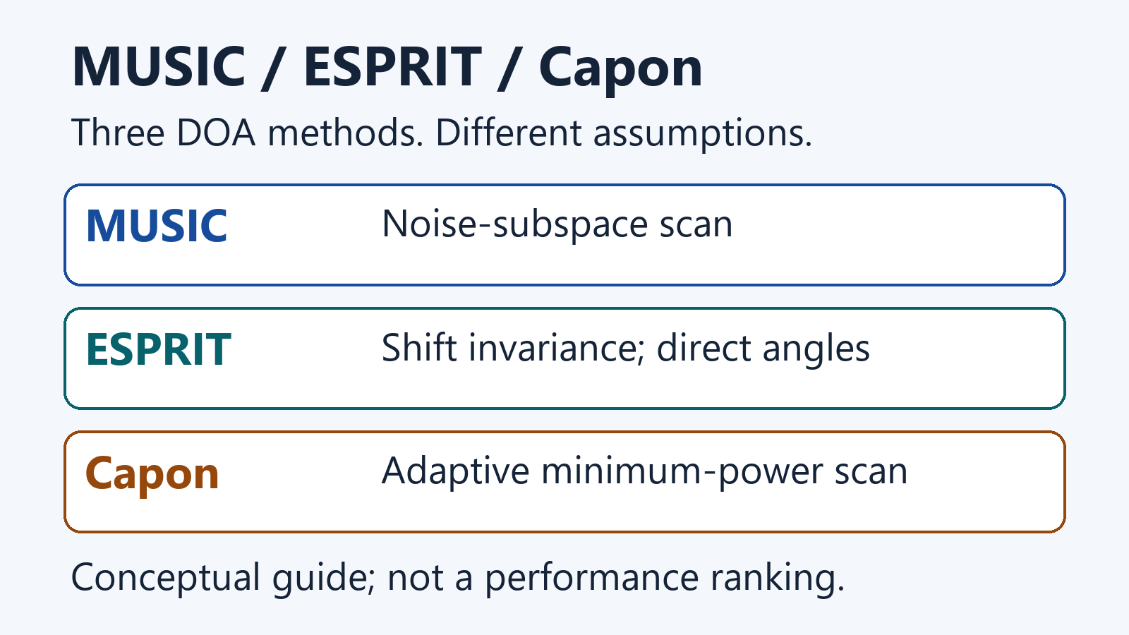
Short answer: choose MUSIC when you have an accurate steering model, a credible source-count estimate, and want an inspectable spatial pseudospectrum. Choose ESPRIT when the array provides matched shift-invariant subarrays and you want direct, gridless angle estimates. Choose Capon when you want an adaptive scanned spectrum, know the steering manifold, and can obtain a well-conditioned covariance estimate. There is no universal accuracy, resolution, or runtime winner.
That recommendation is a synthesis of the methods’ assumptions, not a benchmark ranking. The right choice changes with array geometry, aperture, calibration, source coherence, signal-to-noise ratio, snapshot count, covariance conditioning, scan dimension, and peak-selection policy.
| Method | Best starting point when | Primary constraint | Native output |
|---|---|---|---|
| MUSIC | The steering manifold is accurate and a spectrum is useful | Needs signal-subspace dimension and a scan | Pseudospectrum with peaks |
| ESPRIT | The array has valid matched, translated subarrays | Needs shift invariance and signal-subspace dimension | Direct parameter estimates |
| Capon/MVDR | An adaptive scan is useful and covariance quality is adequate | Needs a known steering manifold, a stable covariance solve, and a scan | Adaptive spatial spectrum |
Scope and prerequisites
This comparison covers snapshot-based direction-of-arrival estimation for narrowband, far-field plane waves whose directions are effectively constant over the observation. It assumes complex sensor samples with their relative phase preserved. Wideband focusing, near-field localization, distributed arrays, and tracking are separate problems.
You should already be comfortable with steering vectors, sample covariance matrices, Hermitian eigendecomposition, and least squares. The data path must retain correctly ordered, synchronized channels; this guide to how to preserve complex multichannel data for angle estimation explains why magnitude-only products are insufficient.
Start with one common array model
Let M be the number of sensors, K the number of sources, and N the number of snapshots, with K smaller than M. For snapshot index n, use the narrowband model
\mathbf{x}[n]=\mathbf{A}(\boldsymbol{\theta})\mathbf{s}[n]+\mathbf{u}[n],\qquad n=0,\ldots,N-1.Here, x[n] is the M-by-1 sensor snapshot; s[n] is the K-by-1 source vector; u[n] is additive noise; the K angles are collected in θ; and A is the M-by-K steering matrix whose columns are steering vectors. Superscript H below means conjugate transpose. Stack the snapshots into the M-by-N matrix X and estimate the covariance as
\widehat{\mathbf{R}}=\frac{1}{N}\sum_{n=0}^{N-1}\mathbf{x}[n]\mathbf{x}^{H}[n]=\frac{1}{N}\mathbf{X}\mathbf{X}^{H}.For a uniform linear array, this article measures θ from broadside and uses a positive phase progression. If adjacent sensors are separated by d metres and the wavelength is λ metres, the steering vector is
\mathbf{a}(\theta)=\left[1,\ e^{\mathrm{j}\mu(\theta)},\ \ldots,\ e^{\mathrm{j}(M-1)\mu(\theta)}\right]^{T},\qquad \mu(\theta)=\frac{2\pi d}{\lambda}\sin\theta.Here, j is the imaginary unit, superscript T means ordinary transpose, and the spatial phase increment is mu. A negative-exponent convention is equally valid, but its phase-to-angle sign must be changed consistently. The derivation of how antenna phase encodes direction of arrival gives more context for this spatial-frequency mapping. The array manifold must be unique over the declared field of view; otherwise different angles can produce indistinguishable steering vectors.
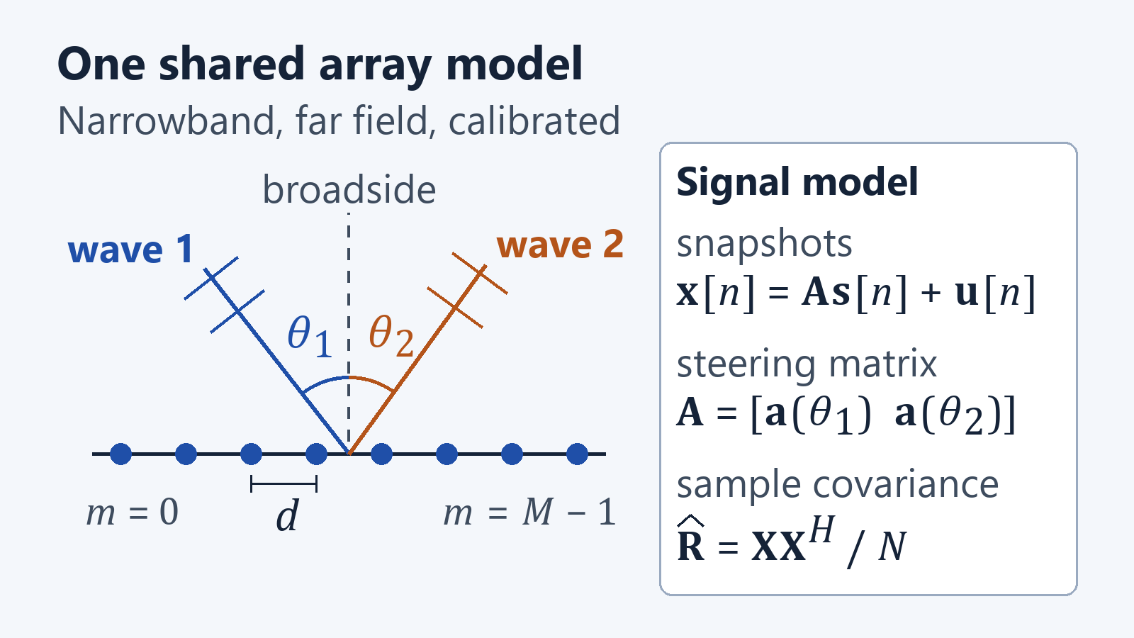
The shared equations hide different requirements. Baseline MUSIC uses a signal/noise subspace split. Baseline ESPRIT adds a shift-invariance requirement. Capon uses a constrained covariance fit at each tested direction. Those differences drive the choice.
MUSIC: search for steering vectors orthogonal to noise
MUSIC eigendecomposes the covariance and divides the eigenvectors into an estimated K-dimensional signal subspace E-s and an (M minus K)-dimensional noise subspace E-n. Under the ordinary spatially white-noise, full-rank source model, a true steering vector is orthogonal to the population noise subspace. The scanned pseudospectrum is
P_{\mathrm{MUSIC}}(\theta)=\frac{1}{\mathbf{a}^{H}(\theta)\mathbf{E}_{n}\mathbf{E}_{n}^{H}\mathbf{a}(\theta)}.The largest peaks are the angle candidates. Exact orthogonality and infinite peaks are population statements; finite data produce finite, perturbed peaks. The original MUSIC paper by Schmidt formulates the method for general calibrated manifolds, including irregular arrays, while the current MUSIC derivation and implementation notes make the sample-covariance, source-count, grid, and correlated-source assumptions explicit.
When MUSIC is a strong fit
- You know or can calibrate the steering vector over the required field of view.
- You can estimate K reliably and want a one- or two-dimensional spectrum for inspection or downstream peak detection.
- The array is not shift-invariant, so standard ESPRIT is unavailable, but a unique manifold is known.
Ordinary grid MUSIC returns peaks on its chosen grid. A denser grid samples the objective more finely but does not enlarge the physical aperture or create information. Root-MUSIC is a distinct gridless variant and is outside this three-method comparison. MUSIC peak heights are also not calibrated source-power estimates.
ESPRIT: turn subarray translation into an eigenvalue problem
Standard ESPRIT uses two matched subarrays related by a known displacement. For an M-element uniform linear array, a common construction takes sensors 1 through M minus 1 for the first subarray and sensors 2 through M for the second. Apply the corresponding selection matrices to the estimated signal subspace and fit a K-by-K rotation operator Ψ:
\mathbf{J}_{2}\mathbf{E}_{s}\approx\mathbf{J}_{1}\mathbf{E}_{s}\boldsymbol{\Psi},\qquad \boldsymbol{\Psi}\mathbf{q}_{k}=\gamma_{k}\mathbf{q}_{k}.J-1 and J-2 select the first and second translated subarrays; q-k is the kth eigenvector of the fitted rotation operator. The eigenvalue γ-k carries the phase shift between the subarrays. For a one-sensor displacement d and the positive-exponent, broadside-angle convention declared above, map that phase to angle by
\widehat{\theta}_{k}=\arcsin\!\left(\frac{\lambda\,\arg(\gamma_{k})}{2\pi d}\right).Phase wrapping and spatial ambiguity still apply, and a different displacement or steering sign changes the mapping. ESPRIT therefore avoids an angular grid; it does not avoid geometry. The Roy and Kailath ESPRIT paper derives the rotational-invariance idea and its assumptions. Current ESPRIT implementation documentation likewise requires a uniform linear array, constructs overlapping translated subarrays, and estimates or accepts the number of signals.
“Calibration-free” is too strong
ESPRIT can avoid storing and searching a complete angle-indexed manifold, but the paired subarrays must still be matched, their displacement must be known, and their channels must have compatible gain, phase, element response, and timing. Violating that invariance biases the rotation estimate. ESPRIT is attractive when the hardware genuinely supplies the structure—not when the structure is merely assumed.
Capon/MVDR: minimize output power under a distortionless constraint
At each tested angle, the Capon construction using total sample covariance (MPDR in the strict terminology below) chooses weights that pass the tested steering vector with unit response while minimizing output power:
\underset{\mathbf{w}}{\operatorname{minimize}}\ \mathbf{w}^{H}\widehat{\mathbf{R}}\mathbf{w}\qquad \text{subject to}\qquad \mathbf{w}^{H}\mathbf{a}(\theta)=1.When the covariance is positive definite, the solution and its scanned spectrum are
\mathbf{w}_{\mathrm{MPDR}}(\theta)=\frac{\widehat{\mathbf{R}}^{-1}\mathbf{a}(\theta)}{\mathbf{a}^{H}(\theta)\widehat{\mathbf{R}}^{-1}\mathbf{a}(\theta)},\qquad P_{\mathrm{Capon}}(\theta)=\frac{1}{\mathbf{a}^{H}(\theta)\widehat{\mathbf{R}}^{-1}\mathbf{a}(\theta)}.This constrained minimum-power interpretation is documented with the weights in the MVDR weight definition, while Capon’s original frequency–wavenumber paper presents the adaptive inverse-spectral-matrix estimator and discusses its invertibility. In software, solve linear systems or use a matrix factorization; an explicit inverse is not required.
Covariance choice and loading must be stated
Terminology is not perfectly uniform. The current beamforming overview distinguishes strict MVDR using a noise-plus-interference covariance from MPDR using a total sample covariance, while current estimator documentation labels the scanned method “MVDR (Capon)”. A reproducible result should name the covariance actually supplied.
If the sample covariance is singular or poorly conditioned, one common regularization is diagonal loading:
\widehat{\mathbf{R}}_{\delta}=\widehat{\mathbf{R}}+\delta\mathbf{I},\qquad \delta>0.I is the M-by-M identity matrix. The loading δ has the same power units as a covariance entry. Positive loading makes a Hermitian positive-semidefinite covariance positive definite, but it changes the estimator. No single loading value is optimal across arrays and scenes. Capon spectrum formation does not require K, but turning that spectrum into a fixed-length DOA list still requires peak detection and a decision about how many peaks to return.
Side-by-side comparison
| Criterion | MUSIC | ESPRIT | Capon/MVDR spectrum |
|---|---|---|---|
| Core operation | Noise-subspace orthogonality | Signal-subspace shift fit | Constrained minimum-power scan |
| Angle scan | Yes, for conventional MUSIC | No | Yes |
| Source count K | Needed to form the noise subspace | Needed to form the signal subspace | Not needed to form the spectrum; needed for a fixed-count peak list |
| Array requirement | Known, unique steering manifold; regular or irregular | Matched shift-invariant subarrays | Known steering manifold and stable covariance solve |
| Returned object | Pseudospectrum; peak magnitude is not source power | Direct angle estimates | Adaptive spectrum; interpretation depends on covariance and normalization |
| Grid error | Present in ordinary grid MUSIC | No angular-grid quantization | Present in the scanned spectrum |
| Typical numerical pressure point | Subspace split and model-order error | Subspace split and invariance mismatch | Covariance conditioning and steering mismatch |
| Coherent sources | Can destroy the assumed source rank | Excluded by the original fully coherent-source derivation | Do not assume immunity; test the exact scene and preprocessing |
Computational structure, not a runtime ranking
For dense straightforward implementations, forming the covariance is on the order of N times M squared operations. An M-by-M eigendecomposition or factorization is on the order of M cubed. With G tested angles, ordinary MUSIC and Capon add grid-dependent work commonly on the order of G times M squared; ESPRIT instead adds a subspace fit and a K-dimensional eigensolve. These are order-of-growth inferences, not timing results. Structure-aware solvers, scan dimensionality, batching, hardware, and implementation details can reverse a wall-clock ranking. A published performance–complexity comparison should therefore be read under its stated arrays, metrics, and simulations, not as a universal leaderboard.
A reproducible synthetic example
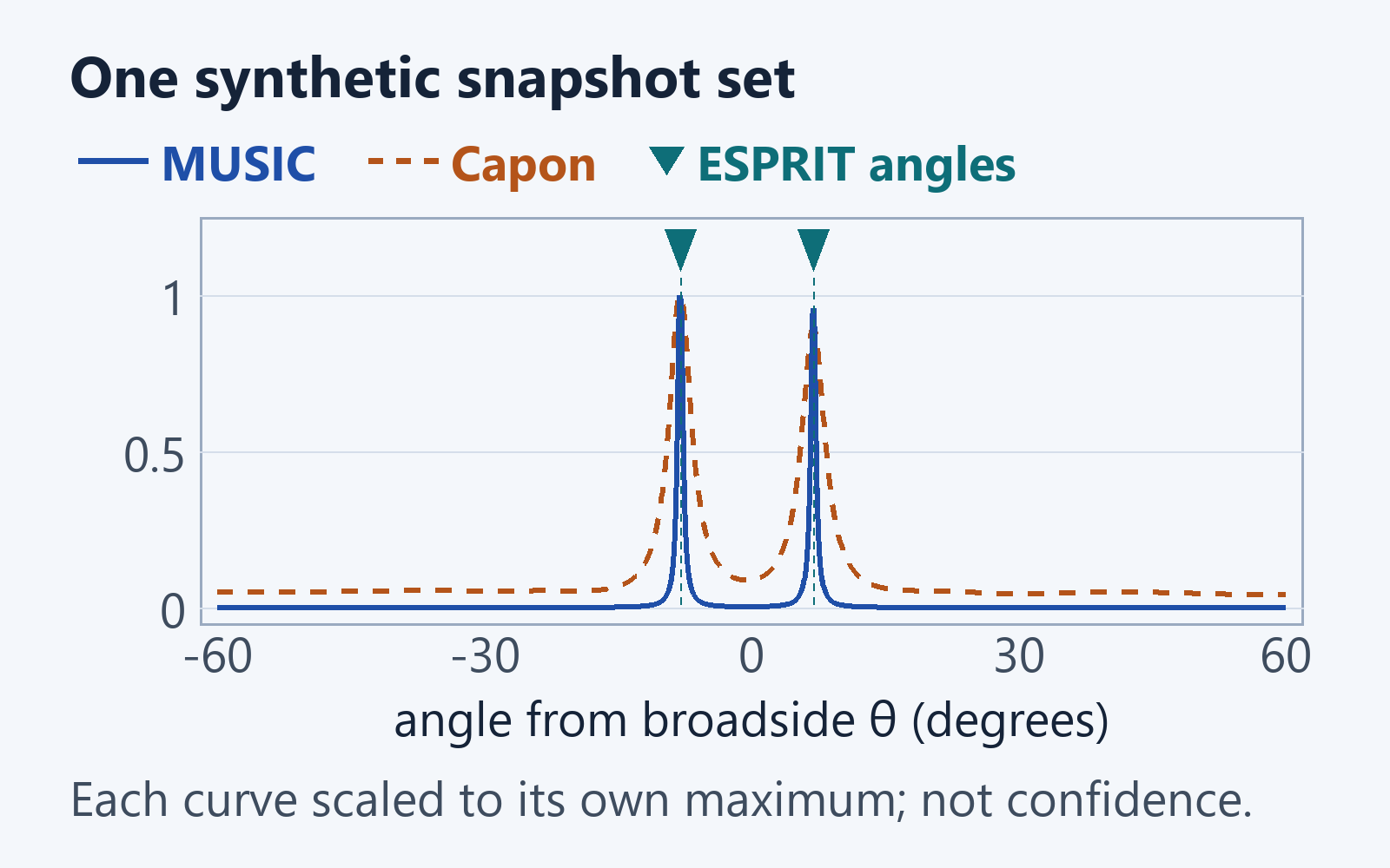
The following calculated example is a consistency check, not a performance benchmark. It uses an ideal ten-element uniform linear array, independent equal-power complex Gaussian sources at −8° and 7°, half-wavelength spacing, 256 snapshots, a nominal aggregate per-sensor SNR of 5 dB, spatially white complex Gaussian noise, and random seed 20261016. MUSIC and ESPRIT receive the true model order K = 2. MUSIC and Capon scan −60° to 60° in 0.05° steps. Capon uses the illustrative loading δ = 0.001 times the mean covariance diagonal; this is not a recommended universal setting.
import numpy as np

rng = np.random.default_rng(20261016)
M, N, K = 10, 256, 2
d = 0.5                       # sensor spacing in wavelengths
truth = np.array([-8.0, 7.0]) # broadside angles in degrees
snr_db = 5.0                  # aggregate signal power / noise power

m = np.arange(M)[:, None]
def steering(degrees):
    angles = np.deg2rad(np.atleast_1d(degrees))
    return np.exp(1j * 2 * np.pi * d * m * np.sin(angles))

A = steering(truth)
S = (rng.standard_normal((K, N)) + 1j * rng.standard_normal((K, N))) / np.sqrt(2)
noise_variance = K / (10 ** (snr_db / 10))
W = np.sqrt(noise_variance / 2) * (
    rng.standard_normal((M, N)) + 1j * rng.standard_normal((M, N))
)
X = A @ S + W
R = X @ X.conj().T / N

eigenvalues, eigenvectors = np.linalg.eigh(R)
Es = eigenvectors[:, -K:]
En = eigenvectors[:, :M-K]

grid = np.arange(-60.0, 60.0 + 0.05, 0.05)
Ag = steering(grid)
music_denominator = np.real(np.sum(Ag.conj() * (En @ En.conj().T @ Ag), axis=0))
music = 1.0 / np.maximum(music_denominator, np.finfo(float).eps)

loading = 1e-3 * np.trace(R).real / M
R_loaded = R + loading * np.eye(M)
capon_denominator = np.real(np.sum(Ag.conj() * np.linalg.solve(R_loaded, Ag), axis=0))
capon = 1.0 / np.maximum(capon_denominator, np.finfo(float).eps)

Psi = np.linalg.pinv(Es[:-1, :]) @ Es[1:, :]
spatial_frequency = np.angle(np.linalg.eigvals(Psi)) / (2 * np.pi * d)
esprit = np.sort(np.rad2deg(np.arcsin(np.clip(spatial_frequency, -1, 1))))

def strongest_local_peaks(spectrum, count):
    candidates = np.flatnonzero(
        (spectrum[1:-1] > spectrum[:-2]) & (spectrum[1:-1] > spectrum[2:])
    ) + 1
    chosen = candidates[np.argsort(spectrum[candidates])[-count:]]
    return np.sort(grid[chosen])

print("truth ", truth)
print("MUSIC", np.round(strongest_local_peaks(music, K), 4))
print("ESPRIT", np.round(esprit, 4))
print("Capon ", np.round(strongest_local_peaks(capon, K), 4))
In the code, W stacks the additive-noise samples u[n]. The retained seed-fixed calculation returns MUSIC angles of −8.00° and 6.95°, ESPRIT angles of −7.9798° and 7.0134°, and Capon peaks at −8.00° and 6.95°. The two scanned methods are quantized to the declared grid. This single favorable, correctly specified run shows implementation consistency only; it cannot establish resolution probability, bias, variance, failure rate, or superiority.
A defensible comparison would repeat many independent trials and vary SNR, snapshots, angular separation, source correlation, calibration error, source powers, model-order policy, grid, loading or smoothing, and failure definition. It would also report the runtime environment. Raw peak height should not be compared across the three methods because MUSIC is a pseudospectrum, ESPRIT returns parameters directly, and Capon’s scale depends on its covariance and normalization.
Failure modes that matter more than the method label
Coherent or strongly correlated sources
Correlation can reduce source-covariance rank, collapsing the subspace dimension MUSIC expects; the original ESPRIT treatment does not cover fully coherent sources. Spatial smoothing on a suitable uniform array can restore useful rank, but each added smoothing step shortens the effective subarray and changes variance and aperture. Current high-resolution DOA guidance treats coherence and smoothing as explicit configuration choices. Do not assume that unmodified Capon is universally immune to coherent multipath.
Too few snapshots or poor conditioning
If N is smaller than M, the ordinary sample covariance has rank at most N and is singular. N at least M is necessary for full rank under generic data, not sufficient for good conditioning. Few snapshots also perturb the eigenvectors used by MUSIC and ESPRIT. Loading, shrinkage, averaging, or a longer observation may help, but each changes the statistical trade-off and must be validated for the intended scene.
Steering mismatch and insufficient aperture
Element-position error, gain/phase mismatch, mutual coupling, antenna-pattern variation, timing offsets, near-field curvature, wideband signals, and motion during the snapshots all break the simple steering model. No estimator can recover angular information that the physical aperture and field of view did not capture. The related radar comparison explains why aperture, geometry, calibration, and processing determine angular capability beyond carrier frequency or channel count.
Model order, grid, and peak policy
An incorrect K changes MUSIC’s and ESPRIT’s estimated subspaces. Capon avoids K while forming the spectrum, not while converting it to a list. Grid spacing, interpolation, minimum peak distance, thresholding, edge handling, and tie-breaking can all change the reported angles. Record these policies as part of the estimator, not as plotting trivia.
A practical decision rule
- Verify the measurement first. Confirm narrowband far-field validity, complex phase preservation, channel order, synchronization, field of view, and a calibrated or otherwise trustworthy array model.
- Use ESPRIT when its geometry is genuinely available. Valid matched translated subarrays, reliable K, and a preference for direct gridless estimates make it the natural candidate.
- Otherwise use MUSIC when manifold-based inspection matters. It supports arbitrary known manifolds and produces an interpretable search surface, but it needs K and a scan policy.
- Use Capon when adaptive scanned power is the desired object. It is especially useful when you do not want K to define the spectrum, provided covariance conditioning, loading, and steering mismatch are controlled.
- Validate at the operating boundary. Test close sources, low SNR, few snapshots, coherent paths, off-axis directions, calibration drift, and model-order or peak-count mistakes. Choose by the failure metric that matters in deployment.
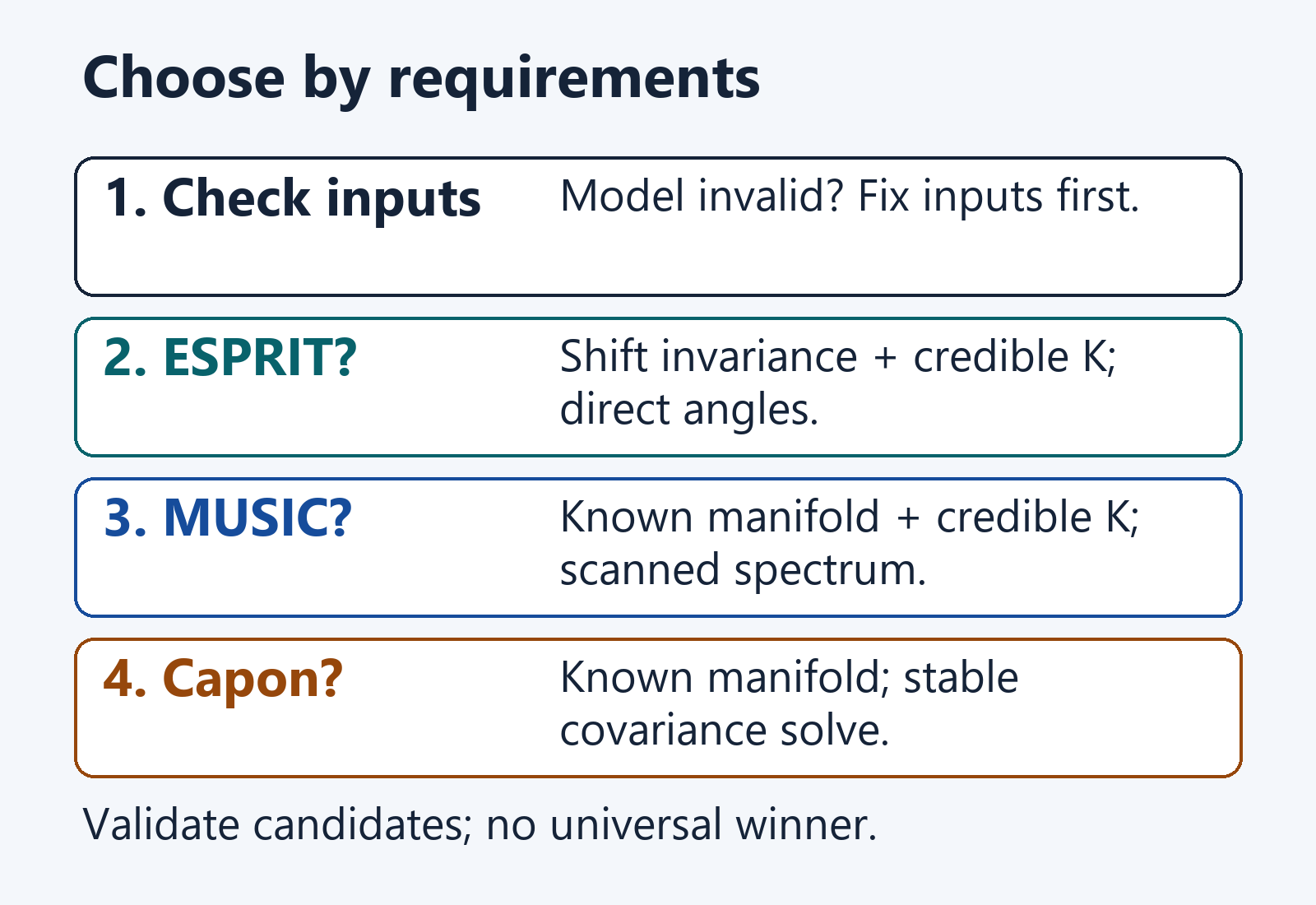
In practice, it is often sensible to implement two methods on the same calibrated covariance pipeline. Agreement under controlled conditions is a useful diagnostic; disagreement is a reason to inspect assumptions, not to average the angles blindly.
Key takeaways
- MUSIC is the flexible manifold-based, scan-and-peak choice; its central risks are model order, finite-sample subspace leakage, and calibration error.
- ESPRIT is the direct gridless choice when matched shift-invariant subarrays really exist; it still needs model order and hardware consistency.
- Capon/MVDR is the adaptive scanned-spectrum choice; it avoids model order during spectrum formation but depends strongly on covariance and steering quality.
- Coherence, few snapshots, mismatch, ambiguity, and peak policy can dominate the nominal algorithmic differences.
- A fair comparison fixes the data, geometry, aperture, preprocessing, and output policy, then reports condition-specific error and failure rates—never a universal winner.
References
- R. O. Schmidt, “Multiple Emitter Location and Signal Parameter Estimation”, IEEE Transactions on Antennas and Propagation, 1986.
- R. Roy and T. Kailath, “ESPRIT—Estimation of Signal Parameters Via Rotational Invariance Techniques”, IEEE Transactions on Acoustics, Speech, and Signal Processing, 1989.
- J. Capon, “High-Resolution Frequency-Wavenumber Spectrum Analysis”, Proceedings of the IEEE, 1969.
- MathWorks, “MUSIC Super-Resolution DOA Estimation”, R2026b documentation.
- MathWorks, “phased.ESPRITEstimator”, R2026b documentation.
- MathWorks, “mvdrweights” and “phased.MVDREstimator”, R2026b documentation.
- MathWorks, “High Resolution Direction of Arrival Estimation” and “Beamforming Overview”, R2026b documentation.
- E. Gentilho Jr., P. R. Scalassara, and T. Abrão, “Direction-of-Arrival Estimation Methods: A Performance-Complexity Tradeoff Perspective”, arXiv:2002.01588v1, 2020.