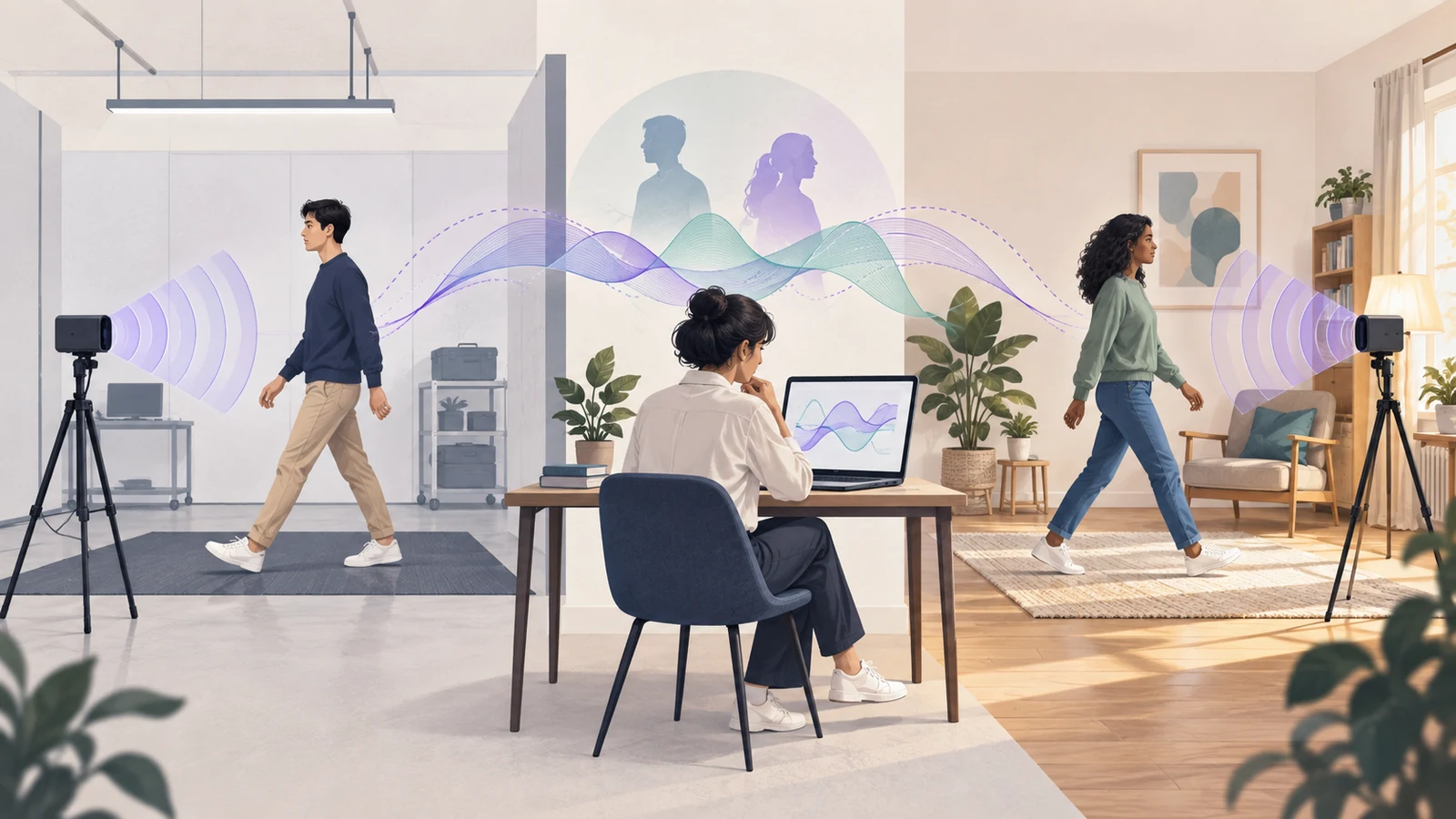
A radar-HAR accuracy of 98% is meaningful only when the test split matches the intended use. Randomly splitting windows can put the same people, recordings or even raw samples into training and testing. A model may then perform well on familiar conditions while struggling with an unseen person, room or radar configuration. To assess generalization, keep the relevant groups separate, protect the test set throughout development, and report performance across people and activities alongside the overall score.
The 98% in this title is an illustrative headline, not a quotation from a particular paper. High accuracy does not establish that an experiment contains leakage. The question is what the experiment allows that number to mean.
This guide explains how to connect a radar human activity recognition (radar-HAR) claim to its evaluation protocol. It includes an overlap calculation, a worked example in which a legitimate 98% average hides weaker results for several people, and a practical split-audit workflow.
Start with the claim behind the percentage
Suppose a paper classifies walking, sitting, standing and other activities from radar spectrograms. Before comparing its accuracy with another model, ask: did the test examples come from new windows, new recordings, new sessions, new people or new environments? These are different experiments.
A personalized system can legitimately learn from its eventual user. A system intended for people who never contributed training data needs a subject-independent test. Neither protocol answers every deployment question. Problems arise when the claim extends beyond the separation that the experiment actually enforced.
Kapoor and Narayanan’s work on leakage in machine-learning-based science connects evaluation errors to unsupported scientific claims. Here, we distinguish information crossing a protected split from a mismatch between the tested population and the claimed deployment. Both can make a headline misleading, but their remedies differ.
How subject leakage happens in radar-HAR
A radar recording reflects an activity performed by a particular person under particular measurement conditions. Walking speed, limb motion, body orientation, range and the surrounding scene can all affect the representation. Our guide to human micro-Doppler explains why the same activity need not produce one universal signature.
When windows from each participant appear in both training and testing, the model can benefit from patterns associated with those familiar participants. This is usually called a subject-dependent evaluation. It becomes subject leakage relative to an unseen-person claim when the reported protocol lets those identities cross the boundary that the claim requires.
Subject identity does not automatically reveal the activity. If every participant performs every class, recognizing a person alone cannot solve a balanced classification task. Familiar participant-specific motion patterns can still make classification easier. A stronger shortcut appears when participant identity, room or recording order also predicts the label—for example, when one group supplies most walking examples and another supplies most sitting examples.
Do not attempt to remove every person-specific feature merely because it exists. Some variation carries useful motion information. Design the evaluation to reveal whether the model can use that information for the population you intend to serve.
Overlapping windows can share the actual test data
Consider a continuous radar recording divided into four-second windows with a one-second hop. One window covers seconds 0–4; the next covers seconds 1–5. They share three seconds of input. For equal windows of duration L and a hop H, with a positive hop no larger than the window, the shared fraction is:
q=\frac{L-H}{L},\qquad 0<H\leq L.Here, the overlap is 3/4, or 75%. If random window splitting places the first window in training and its neighbour in testing, the test input is partly reused training data. The filenames and window indices can differ even though most of the measurement interval is identical.
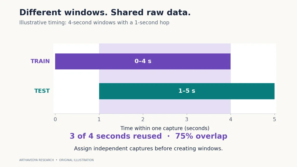
Overlap is useful for frequent predictions and can be a reasonable training choice. The problem is overlap across partitions that are supposed to be independent. Keep all windows from an independent capture together. For a chronological protocol that deliberately divides one long stream, account for the complete input support on each side, including filtering, spectrogram frames and model context; a nominal timestamp boundary alone may not prevent sample reuse.
Dehghani, Glatard and Shihab’s 2019 study of subject cross-validation demonstrated evaluation inflation from sample-wise validation and overlapping windows in wearable-sensor HAR. It provides evidence for the dependence problem, rather than a numerical estimate of how much a particular radar result is inflated. An overlap percentage is also not an accuracy-inflation percentage.
The same provenance rule applies to augmented copies, alternative spectrogram settings and synchronized views of one event. Noise-augmented training data must not descend from a held-out test recording. If multiple radar sensors observe the same activity trial, keep that shared event together for an independent-event evaluation. A paired sensor-transfer experiment may deliberately use corresponding events, but it must state that narrower protocol.
Choose a split that can support your claim
| Intended claim | What stays outside training and model selection | What the result still does not establish |
|---|---|---|
| New recordings of familiar people | Entire independent recordings or trials | Performance on people absent from development |
| The same people on a later day | Later sessions, with the intended time order respected | Unseen-person or unseen-room performance |
| New people in familiar settings | All recordings of the held-out participants | Transfer to a room or device never encountered |
| New rooms with familiar people allowed | All data from the held-out rooms | Unseen-person performance |
| New people in new rooms | Both the test participants and test rooms | Transfer to every possible population or environment |
| A different radar configuration | The target configuration, except for explicitly allowed adaptation data | Independent-event transfer if paired captures cross the boundary |
Leave-one-subject-out (LOSO) holds out one participant for evaluation and repeats this across participants. Group k-fold holds out groups of participants in each fold. A fixed participant-disjoint train/validation/test split is another valid design. The appropriate choice depends on the study size, tuning budget and deployment question; LOSO is not automatically the most precise estimate.
Stratification and grouping solve different problems. Stratification aims to preserve class proportions. Grouping prevents the same participant or other chosen unit from appearing on both sides. A stratified random split of windows remains subject-dependent. The scikit-learn grouped-validation documentation describes the corresponding splitters and their constraints.
A subtle trap: grouping by person–room pairs
Suppose the groups are “Person 1 in Room A” and “Person 1 in Room B.” A group-aware splitter can keep each pair intact while assigning one pair to training and the other to testing. Person 1 still appears on both sides. Likewise, different people in Room A can enter different partitions while the room remains shared.
A composite person–room identifier therefore tests held-out combinations, not necessarily unseen people and unseen rooms. For a joint claim, enforce each boundary separately. Training participants and test participants must be disjoint; training rooms and test rooms must also be disjoint. Apply the same protection against validation data used for tuning.
If held-out test participants also have recordings in training rooms, those recordings cannot enter development for an unseen-person claim. If test rooms contain other participants, those recordings cannot enter development for an unseen-room claim. Some collected combinations may consequently remain unused in that particular experiment.
This is easier to plan before recording. The radar-HAR dataset collection guide connects participant, room and session coverage to the claims the dataset can support. When choosing existing data, check these identifiers in the radar-HAR dataset comparison before choosing a network.
Protect the entire pipeline, not just the neural network
Holding out people at the final classifier is insufficient if earlier steps learned from their test data. Dataset-wide scaling, feature selection, dimensionality reduction, learned denoising and representation pretraining can all expose information before the final model is fitted. The scikit-learn leakage guidance recommends splitting first and learning preprocessing parameters from training data only.
| Pipeline decision | Defensible handling |
|---|---|
| Window generation and augmentation | Assign source groups first. Every derived sample inherits the source partition. |
| Dataset-level mean, variance or PCA | Fit on training data in each fold; apply the fitted transform to validation and test inputs. |
| Fixed FFT or STFT transform | A predetermined per-recording transform can be precomputed if its input support stays within the assigned partition. |
| Per-window normalization | It may use that window’s available input if deployment allows the same operation. Do not include future data in a real-time claim. |
| Empty-room or device calibration | State what target-site data calibration uses and when it is available. Evaluate with the same access policy. |
| Window length, range gate, CFAR settings or confidence threshold | Choose using training/validation evidence. Trying settings until test accuracy improves is test-set tuning. |
| Checkpoint, early stopping and model family | Select using validation groups. Preserve the outer test groups for evaluation. |
The processing choices themselves can change what reaches the model. Our STFT parameter guide and raw-ADC-to-activity pipeline explain those transformations. In an evaluation study, keep their selection procedure inside the development protocol.
An unlabeled test input still contains information. If a pretrained encoder, batch-normalization update or self-supervised objective uses target examples, describe that access. It may be legitimate adaptation, but it changes the experiment from one in which the target data remain unseen until prediction.
Use grouped validation inside grouped testing
For an illustrative study with 12 participants, one fixed design assigns eight people to training, two to validation and two to testing. These counts explain separation; they are not a recommendation that 12 people establish adequate population coverage. Both held-out test people remain outside normalization fitting, architecture selection and early stopping.
If the study instead uses outer LOSO evaluation, perform model selection using only the remaining participants in each outer fold. Inner validation must also keep the relevant groups separate. After choosing the configuration, fit the allowed development data and evaluate the outer held-out participant. Repeat the complete procedure for each outer fold.
Varma and Simon’s analysis of cross-validation used for model selection shows why using the same validation results to select a model and report its performance creates optimistic estimates. Nested evaluation separates those roles. It does not require an exhaustive search; a small, declared candidate set can be more practical.
Comparing random-window and participant-disjoint scores can be informative, but their difference is not a direct measurement of leakage. The training population, training-set size and test difficulty may also change. For model comparisons, use the same predefined outer splits, comparable tuning budgets and matched evaluation rules. Report repeated seeds as training variability, not as additional independent participants.
Domain shift can remain after leakage is removed
Domain shift means that the data encountered at the target differ from the training conditions. A clean split prevents a particular form of contamination; it does not make a new room or sensor statistically equivalent to the old one.
- Viewing direction and placement: Doppler reflects radial motion. A side-on walk can look different from a walk toward the radar; range and mounting height also change the observed body and geometry.
- Room and background: multipath, static reflectors, moving clutter and occlusion can alter the measured signature.
- Radar configuration: bandwidth, chirp timing, frame rate, array geometry and processing thresholds can change resolution, coverage and point-cloud density. Equal tensor dimensions do not guarantee equal physical information.
- People and behaviour: pace, mobility, carrying objects and natural transitions may differ from rehearsed laboratory actions.
- Label definitions: “sitting” can mean the seated state in one dataset and the sit-down transition in another. Compare the annotation rules before treating their labels as equivalent.
What a radar adaptation study actually demonstrates
Hernangómez and colleagues studied activity classification across four 60-GHz FMCW radar configurations, using recordings of two male participants performing five activities. Their EUSIPCO 2022 work reports configuration-transfer accuracies from 85.8% to 92.5% with Margin Disparity Discrepancy and unlabeled target-domain data (experimental setup and Table II).
That is evidence about a specified adaptation problem. It is not a test of zero-access transfer to every new person and home. The study also explains that resampling inputs to matching dimensions did not remove the configuration differences. This is a useful warning against assuming that resizing a spectrogram solves the underlying measurement shift.
Declare the target-data access policy
| Evaluation setting | Permitted target information before final scoring |
|---|---|
| Domain generalization / no target adaptation | No target-domain samples used to learn or select the system. |
| Unsupervised domain adaptation | Unlabeled target inputs; declare whether the eventual evaluation inputs themselves are included. |
| Supervised or few-shot adaptation | A specified labeled target adaptation set, kept separate from final evaluation events. |
| Online adaptation | Only the stream history and information available by each prediction time, under a declared update rule. |
Using unlabeled final evaluation inputs for adaptation is a transductive protocol. It can be a legitimate research setting, but it does not measure performance on a completely unseen future target batch. State the target sample budget, calibration procedure, label access and event overlap so readers can identify the claim.
These distinctions also matter when comparing sensing technologies. Our evidence-led comparison of radar and cameras for human monitoring shows why a sensor comparison needs matched tasks and evaluation conditions.
A clean 98% can still hide weaker users
Leakage is not the only reason to look beyond overall accuracy. Imagine the following synthetic counting example for four held-out participants. These are invented counts for teaching the averaging calculation, not measured radar predictions.
| Test participant | Test windows | Correct predictions | Accuracy |
|---|---|---|---|
| A | 9,000 | 8,910 | 99% |
| B | 500 | 475 | 95% |
| C | 300 | 255 | 85% |
| D | 200 | 160 | 80% |
| Total | 10,000 | 9,800 | 98% pooled |
Pooled window accuracy gives every window equal weight. Participant-averaged accuracy first calculates accuracy for each person and then gives each person equal weight. With S test participants, ns windows and cs correct predictions for participant s:
A_{\mathrm{window}}=\frac{\sum_{s=1}^{S}c_s}{\sum_{s=1}^{S}n_s}.A_{\mathrm{person}}=\frac{1}{S}\sum_{s=1}^{S}\frac{c_s}{n_s}.The first calculation gives 98%. The second gives 89.75%, the mean of 99%, 95%, 85% and 80%. Both calculations are correct. They answer different weighting questions, and the 98% aggregate largely reflects Participant A.
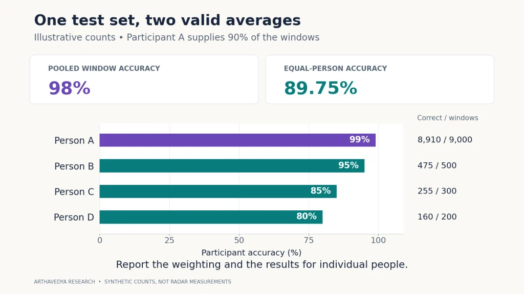
Neither weighting is universally preferable. Window weighting may reflect an operational stream when recording duration matches intended use; equal-person weighting makes variation across users more visible. Report both when they answer relevant questions, together with participant counts and the per-person distribution. Also check activity coverage within each person: changing the weighting across people does not automatically balance the activities.
Report class performance and uncertainty separately
A system that misses a less frequent activity can retain high overall accuracy. Macro-F1 gives each declared class equal weight after computing its F1 score. For class k, true positives (TP), false positives (FP) and false negatives (FN) give:
F_{1,k}=\frac{2\mathrm{TP}_k}{2\mathrm{TP}_k+\mathrm{FP}_k+\mathrm{FN}_k}.F_{1,\mathrm{macro}}=\frac{1}{K}\sum_{k=1}^{K}F_{1,k}.Here, K is the number of evaluated activity classes. Macro-F1 is the mean of class F1 scores; it is not the F1 calculated from averaged precision and recall. Declare the class list and how undefined scores are handled. A fold lacking examples of an activity supplies no evidence about recall for that activity; silently dropping absent classes can make fold averages incomparable. The scikit-learn classification-metric definitions describe these averaging and zero-division conventions.
| Report | What it helps the reader assess |
|---|---|
| Overall accuracy and macro-F1 | The aggregate result and performance across classes. |
| Confusion matrix, class recall and class support | Which activities are confused and how much evidence supports each rate. |
| Per-person and per-domain results | Whether a strong average hides weak participants, rooms or configurations. |
| Participants, sessions, trials and windows | How many separate units produced the nominal sample count. |
| Uncertainty method and repeated-seed results | Sampling uncertainty and training instability as separate sources of variation. |
| Event errors and detection delay for continuous use | Whether a window classifier produces useful behaviour after smoothing and alert logic. |
Ten thousand windows are not ten thousand independent people
Errors from overlapping windows or repeated trials of one participant can be correlated. Treating them as independent Bernoulli trials can make confidence intervals appear too narrow. Repeating a split or changing a random seed does not add new population coverage.
For uncertainty across new users, one practical analysis resamples held-out participants as clusters and keeps each selected participant’s windows together. For a paired comparison between models, resample the same participants for both. State the estimand—such as equal-person accuracy—and the resampling scheme. If people share sessions or environments, those dependencies may require a richer hierarchical analysis.
A participant bootstrap over fixed test predictions does not include all uncertainty from retraining or selecting a model. With very few independent test participants, bootstrap intervals are themselves fragile. Report the individual results and the coverage limitation. Varoquaux’s work on cross-validation uncertainty cautions that fold-to-fold standard errors can understate uncertainty; that study is about neuroimaging, not a radar-specific confidence interval formula.
A practical workflow before the next training run
- Write the deployment claim. Identify what will be new: person, session, room, device, configuration or several of these. Specify whether target calibration or adaptation is allowed.
- Create a provenance manifest. Record subject, session, recording, shared capture/event, environment and configuration identifiers. Retain each sample’s source and full input-support interval. Give synchronized sensor files one shared capture identifier.
- Assign independent groups. Choose train, validation and test membership before inspecting model results. Inherit membership when creating windows or augmentations. Check class coverage without selecting splits for favourable accuracy.
- Audit every boundary. Compare group identifiers across partitions; check duplicate content and raw-time overlap. For a joint claim, test each required axis separately. Reject missing or ambiguous provenance instead of treating missing IDs as unique people.
- Fit and select inside development. Learn preprocessing on training folds. Use grouped validation to select parameters, checkpoints and thresholds. Preserve the outer evaluation protocol.
- Score and report the declared task. Include pooled, per-class and per-person results where relevant. Separate no-adaptation and adaptation results. Save split manifests, seeds, software versions and exclusion rules.
The companion Python tool audits a CSV manifest and reproduces the two illustrative figures. Its default audit requires capture-disjoint partitions and checks participant separation. Repeated --holdout arguments add independent boundaries, such as environment. It also checks recording IDs, optional augmentation-lineage IDs, optional SHA-256 sample hashes, class coverage and cross-partition overlap in the declared raw input intervals.
python radar_har_evaluation_tools.py demo --output-dir evaluation-demo

python radar_har_evaluation_tools.py audit manifest.csv \
  --holdout subject_id --holdout environment_id \
  --output-json audit.json
An audit pass means that the supplied metadata passed those checks. It cannot verify that IDs are truthful, discover undisclosed preprocessing fitted on test data, or establish that the study population represents deployment. The tool deliberately flags whole-capture reuse, so a paired sensor-transfer or same-stream chronological study needs its own declared audit policy rather than an exception hidden in the manifest.
What to do when the stronger test score falls
First check implementation errors, inconsistent label definitions and unexpected preprocessing changes. Then inspect the difficult participants and domains. A score drop after changing the split can reflect several factors at once; it is not evidence that a particular network learned only identity.
If subject variation dominates, improve participant coverage and examine class performance across users. If viewing direction dominates, collect or test the relevant geometry. If configuration differences dominate, preserve physical axis meanings and evaluate an explicitly defined transfer or adaptation method. Keep the stronger test as evidence about the problem you actually need to solve.
Do not select a more favourable split to restore the headline. If you inspect the test errors and use them to redesign the system, that test has become development evidence. A revised performance claim then needs a fresh holdout or a newly defined outer evaluation that accounts for the selection process.
What a credible 98% claim includes
A credible result identifies the prediction task, held-out unit, population and measurement conditions, target-data access, selection procedure and weighting behind the metric. It shows which people and activities remain difficult, and it distinguishes a laboratory classification result from continuous operation.
The goal is a score that answers the deployment question. For an unseen-user claim, that starts with unseen users. For an unseen-room claim, it starts with unseen rooms. Better models matter after the evaluation boundary is clear.
References
- Kapoor, S., and Narayanan, A. Leakage and the reproducibility crisis in machine-learning-based science. Patterns, 2023. Authors’ project, paper link and leakage taxonomy.
- Dehghani, A., Glatard, T., and Shihab, E. Subject Cross Validation in Human Activity Recognition. arXiv:1904.02666v2, 2019. Original preprint. Wearable-sensor HAR; cited for the validation mechanism.
- Hernangómez, R., Bjelaković, I., Servadei, L., and Stańczak, S. Unsupervised Domain Adaptation across FMCW Radar Configurations Using Margin Disparity Discrepancy. EUSIPCO, 2022. Accepted-paper manuscript; published DOI.
- Varma, S., and Simon, R. Bias in error estimation when using cross-validation for model selection. BMC Bioinformatics 7, 91, 2006. Original paper.
- Varoquaux, G. Cross-validation failure: small sample sizes lead to large error bars. Author manuscript, 2017. Neuroimaging methods; cited for uncertainty and dependent fold estimates.
- scikit-learn documentation. Cross-validation for grouped data and GroupShuffleSplit.
- scikit-learn documentation. Common pitfalls: inconsistent preprocessing and data leakage.
- scikit-learn documentation. Classification metrics, class averaging and score conventions.