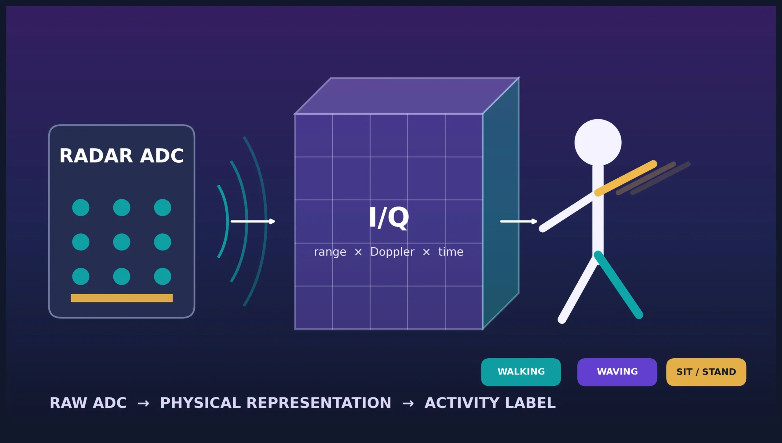
To build a radar-HAR (human activity recognition) pipeline from raw FMCW ADC samples, keep one explicit contract from acquisition to evaluation: validate the capture, decode complex I/Q into a known tensor order, transform fast time into range, transform repeated same-transmitter chirps into Doppler, construct a time-aware learning example, align it with a defensible label, and split independent recordings before creating overlapping windows.
The order matters. A classifier cannot repair missing packets, swapped I/Q, mixed transmitter chirps, a mislabeled transition, or training–test leakage. It may still report excellent accuracy—because those mistakes can create shortcuts that are easier to learn than human motion.
This is the implementation companion to our broader guide on what researchers should decide before starting radar-based human activity recognition. Here the focus is narrower and more practical: what each processing stage receives, what it should output, how to verify it, and where activity labels actually enter the pipeline.
Short answer: do not begin with a neural network. First prove that one known motion survives every transformation from ADC words to a physically calibrated range–Doppler sequence. Then attach labels and enforce group-exclusive evaluation. The model comes after the measurement chain is trustworthy.
The pipeline we are going to build
A useful implementation has five boundaries:
- Capture and verify: preserve ADC words, radar configuration, timestamps and packet-quality information.
- Decode and reshape: reconstruct complex samples in a declared order such as frame, chirp, receiver and fast-time sample.
- Process the radar signal: apply range and Doppler processing with calibrated physical axes and task-appropriate clutter handling.
- Construct learning examples: create range–Doppler sequences, range-gated micro-Doppler, point sets or another representation without hiding preprocessing decisions.
- Align labels and evaluate: associate examples with activity intervals and independent group identifiers before training a baseline.
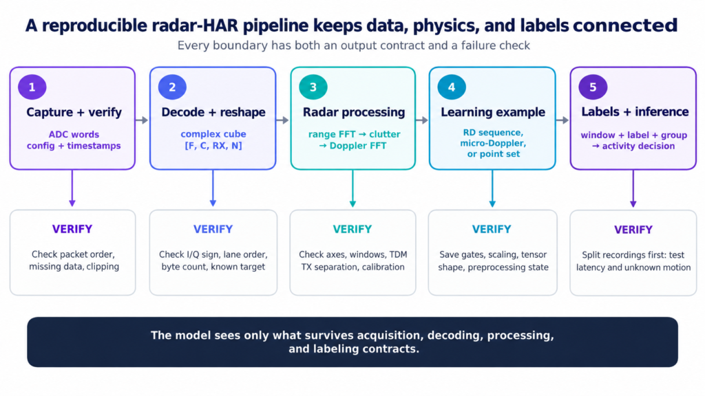
The sections below expand those five boundaries into eight concrete steps. The central engineering principle is simple: every stage needs both an output contract and a verification test. Saving only the final heat maps makes it difficult to determine whether a later failure came from the sensor, decoder, FFT axes, labels or model.
Step 1: freeze the acquisition contract
Raw ADC data is meaningful only together with the configuration that generated it. At minimum, retain the carrier frequency, chirp slope, ADC sampling rate, ADC start time, samples per chirp, chirps per frame, frame period, enabled transmitters and receivers, ADC bit depth, real or complex mode, lane arrangement, I/Q order, sensor orientation and capture-tool version.
Also distinguish three files that are often confused:
- A packetized network capture may contain headers, sequence numbers and missing or out-of-order packets.
- A reordered and zero-filled binary may contain only ADC payload in the device-specific lane order.
- A processed array may already have been decoded, reshaped, calibrated or transformed.
For the Texas Instruments DCA1000 workflow, TI states that Ethernet packets can arrive out of order or be missing, and describes a packet-reorder and zero-fill stage that converts adc_data_RAW_0.bin into the payload file adc_data.bin. TI also warns that packet delay trades streaming throughput against the probability of drops at the host. Those details are not administrative trivia: inserted zero regions can become structured artefacts after Fourier processing. See TI’s raw ADC interpretation report and DCA1000EVM user guide.
Estimate the data rate before recording
For complex 16-bit I/Q, one sample for one receiver occupies four bytes: two for I and two for Q. If a recording has F frames, C total chirps per frame, R enabled receivers and N ADC samples per chirp, its ideal payload size is
V = F C R N b_{\mathrm{IQ}}, \qquad b_{\mathrm{IQ}}=4\ \text{bytes for complex int16}.Consider a single-transmitter example with 20 frames/s, 128 chirps per frame, four receivers and 256 samples per chirp. The ADC payload is 10,485,760 bytes/s, or exactly 10 MiB/s, before packet headers, configuration files or derived representations. A ten-minute session is therefore about 5.86 GiB. Calculate this before choosing the frame count, experiment duration and storage layout.
| Capture check | What to record | Failure symptom |
|---|---|---|
| Expected byte count | Frames, chirps, receivers, samples and bytes per complex sample | Reshape failure, partial frame or silently truncated recording |
| Packet continuity | Sequence counters, missing-byte count and zero-fill report | Repeated stripes, bursts or abrupt gaps after FFT processing |
| ADC headroom | Peak code, clipped-sample fraction and per-channel RMS | Broad spectral energy and distorted amplitudes |
| Configuration identity | Exact configuration file and a hash or immutable run ID | Correct-looking plots with incorrect physical axes |
| Timing | Frame timestamps and label-source timestamps | Actions shifted relative to their labels |
If you are still selecting hardware, the guide to choosing 24, 60 or 77 GHz radar for human sensing explains why raw-data access, usable bandwidth and timing matter more than the frequency label alone.
Step 2: decode the bytes into one canonical radar cube
The decoder’s job is not merely to load integers. It must reconstruct complex samples and assign every value to the correct frame, chirp, receiver and fast-time position. A convenient canonical contract is
x[f,c,r,n]=I[f,c,r,n]+jQ[f,c,r,n].
Here f indexes frames, c indexes transmitted chirps within a frame, r indexes receive channels and n indexes ADC samples within one chirp. In code, document the shape explicitly:
# Canonical contract used by the companion script
adc_cube.shape == (frames, chirps_per_frame, num_rx, adc_samples)
adc_cube.dtype == complex64
Do not assume that every .bin file stores alternating I and Q values. Format depends on the radar family, capture card, number of lanes, real or complex mode, interleaving and I/Q-swap setting. For example, TI documents a two-lane xWR16xx/IWR6843 complex format in which two I values are followed by two Q values. The companion decoder implements that one declared case after packet reordering; it deliberately rejects incomplete frames instead of guessing.
Four decoder tests that catch most errors
- Count test: the number of reconstructed complex samples must equal frames × chirps × receivers × samples.
- Known-target range test: a corner reflector or other isolated target at a measured distance should peak near the predicted range after calibration.
- Channel test: receiver channels should not be accidental duplicates, all zeros or implausibly different in power.
- Motion-sign test: a target moving in a known radial direction should appear on the expected side of the Doppler axis under the declared sign convention.
A heat map that “looks active” is not enough. Wrong lane order can still produce visually complex energy while destroying range and phase relationships.
Step 3: transform fast time into range
For each chirp and receiver, remove only the hardware offset that your method declares, apply a fast-time window, and compute a range FFT across the ADC-sample axis. A Hann window reduces sidelobes, but it also broadens the main lobe and changes amplitude scaling. Save the window choice rather than treating it as a plotting detail.
For the full signal derivation, see how an FMCW chirp becomes a range–Doppler map.
For an ideal linear FMCW chirp with slope S, ADC sampling rate Fs and range-FFT length NR, positive beat-frequency bin k maps approximately to
R_k \approx \frac{c_0 F_s}{2 S N_R}\,k,where c0 is the propagation speed. This is a bin-location formula. The ideal ability to resolve two nearby ranges is governed primarily by the sampled chirp bandwidth B:
\Delta R \approx \frac{c_0}{2B}.Zero-padding from N ADC samples to a larger NR creates more plotted bins and can help locate a peak between the original samples. It does not create new physical range resolution. TI’s chirp-parameter application report develops the relationships among sweep bandwidth, measurement range, velocity and timing.
A concrete 60 GHz example
Suppose the ADC records 256 samples at 5 MS/s during a 75 MHz/µs linear slope. The sampled sweep spans 3.84 GHz, giving an ideal range resolution of about 3.90 cm. With a 256-point range FFT, the range-bin spacing is also about 3.90 cm; with a 512-point FFT it becomes about 1.95 cm, but the underlying 3.90 cm resolution has not doubled.
Step 4: transform slow time into Doppler
After range processing, select one range bin and follow its complex value across repeated chirps. That chirp-to-chirp phase sequence is slow time. Apply the Doppler window and FFT along this axis—not along the ADC-sample axis.
If Ts is the interval between samples from the same transmitter and the Doppler FFT has ND bins, a centered Doppler bin ℓ maps to radial velocity approximately as
\begin{aligned}
f_{D,\ell} &= \frac{\ell}{N_D T_s},\\
v_\ell &= \frac{\lambda f_{D,\ell}}{2},\\
\Delta v_{\mathrm{bin}} &= \frac{\lambda}{2N_D T_s}.
\end{aligned}
When ND is larger than the number of observed chirps, the last expression is displayed bin spacing, not independent physical velocity resolution. As with range zero-padding, more FFT samples interpolate the spectrum without extending the coherent observation.
The TDM-MIMO trap
With time-division multiplexed transmitters, consecutive chirps may come from different antennas. If two transmitters alternate, the interval between chirps from transmitter 1 is approximately twice the single-chirp period. Separate the transmitter sequences before the Doppler FFT. Treating all alternating chirps as one slow-time sequence can corrupt the velocity axis and mix transmitter-dependent phase.
The companion implementation reshapes total chirps into loop and transmitter axes, performs the Doppler transform across loops, and noncoherently sums power across channels. It does not claim calibrated angle estimation. Forming a virtual array for angle processing introduces array-order, channel-calibration and motion-compensation requirements; TI’s MIMO radar report provides the hardware background.
Clutter removal is a task decision
Subtracting the chirp-wise mean of each range bin removes the zero-Doppler component within a frame and often makes motion easier to see. It can also suppress stationary presence, posture information and very slow movement. A fall detector may benefit from moving-target emphasis; a standing-versus-empty or breathing task may not. Report whether clutter subtraction was applied, along which axis, and whether it was fitted per frame, per recording or from separate background data.
Step 5: choose what the model will see
The range–Doppler cube is not automatically the best learning input. The correct representation depends on which physical differences separate the activities and what compute, bandwidth and latency the final system can afford.
| Representation | Preserves | Useful when | Main loss or risk |
|---|---|---|---|
| Complex ADC or range cube | Amplitude and phase before aggressive detection | The signal processing itself is part of the research question | Large, hardware-specific and easy to overfit |
| Range–Doppler sequence | Range, radial velocity and their change over frames | Translation and limb velocity both matter | Higher-dimensional input and configuration dependence |
| Range-gated micro-Doppler | Velocity distribution over time | Motion dynamics matter more than detailed location | Range integration can mix people, clutter or reflectors |
| Point cloud | Detected position, velocity and intensity-like attributes | Spatial motion or lightweight edge output is central | CFAR and firmware have already discarded subthreshold returns |
| Tracks or engineered features | Compact trajectories and selected statistics | Compute, interpretability or data volume is constrained | Potentially useful fine structure is removed by design |
These are different exit points from the processing chain, not interchangeable file extensions. TI’s mmWave SDK data-path overview, for example, distinguishes the ADC buffer, radar cube, detection matrix and detected point cloud. If a device exports only points, thresholds have already shaped the evidence available to the activity model.
Micro-Doppler can make limb motion interpretable, but its appearance depends on viewpoint, velocity resolution, range gating and temporal parameters. See the physics-first guide to how radar sees human micro-Doppler and the practical guide to choosing STFT parameters for radar spectrograms.
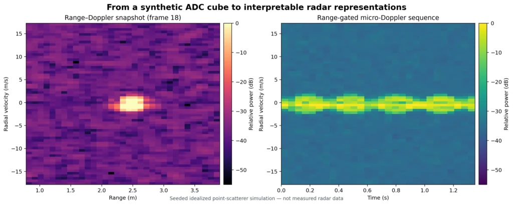
A range-gated micro-Doppler slice can be constructed by summing range–Doppler power over a declared target gate. The gate may be fixed for a controlled single-person setup or follow a detector or tracker. Either way, save its limits. An automatically tracked gate is part of the evaluated algorithm, not invisible preprocessing.
The companion figure uses a seeded idealized point-scatterer signal to verify that the software produces calibrated range–Doppler and time–velocity axes. It is not measured radar data, and its deliberately simple activity classes must not be used as evidence of recognition performance.
Step 6: align activity labels in time
An activity label does not originate in the radar FFT. It comes from an annotation source: a scripted protocol, button press, video, depth camera, motion-capture system, wearable or human review. The pipeline must map that source’s time base to radar frames.
Store labels as intervals when possible, not only as filenames. A useful annotation table contains:
recording_id,start_time_s,end_time_s,label,subject_id,session_id,room_id
rec_0042,3.18,5.74,sit_to_stand,S07,session02,roomA
rec_0042,5.74,7.10,transition,S07,session02,roomA
For every processed window, define one labeling rule before examining model performance. Common choices include the center-frame label, majority temporal overlap, a required purity threshold, multi-label targets, or rejection as a transition. None is universally correct. The important point is that a window containing 55% walking and 45% sitting should not silently become a clean walking example.
Synchronization error should be compared with the motion timescale. A 50 ms offset may be unimportant for a long stationary posture but material for a short gesture or fall onset. A recent 60 GHz motion dataset, for example, reports its radar and skeleton frame rates, timestamp-matching method and residual synchronization errors rather than treating aligned labels as exact. That level of reporting makes downstream claims easier to interpret. See Guo, Dogu and Rajab (2026).
Keep background, transition and unknown labels
A model trained only on pre-cut actions learns closed-set clip classification. A continuous system also sees empty scenes, entry and exit, partial activities, natural transitions, unrelated movements and people doing something outside the vocabulary. Preserve those intervals during collection. Otherwise the deployment problem has been removed from the dataset rather than solved by the model.
Step 7: split independent groups before windowing
This is the most important data-engineering rule in the workflow:
Assign complete recordings, sessions or participants to training, validation and test groups first. Create sliding windows separately inside each group.
If 90%-overlapping windows are created first and then shuffled, nearly identical samples from one event can enter both training and test sets. The nominal sample count grows, but the number of independent human motions does not. Augmented versions of one recording must inherit the same group.
Choose the grouping variable to match the claim:
| Claim | Minimum held-out group | What remains untested |
|---|---|---|
| New clips from known people | Recording or session | Unseen-person generalization |
| Works for new users | Participant | New rooms, viewpoints and devices |
| Works in new rooms | Environment | Unseen hardware or activity classes |
| Transfers across sensors | Device or configuration | Other populations and environments |
The Google Soli study is instructive here. Its authors explicitly avoided randomly mixing highly correlated samples and used separate sessions, yet the same five participants appeared in training and testing. The result therefore tested session repeatability for known users, not universal unseen-user recognition. Our breakdown of what Google Soli actually proved examines that boundary in detail; the original paper provides the experiment.
For a software baseline, a group-aware splitter is safer than ordinary random cross-validation. Scikit-learn’s StratifiedGroupKFold documentation defines stratified folds with non-overlapping groups. The companion script uses subject identifiers for this purpose and keeps session identifiers in the feature table.
Step 8: establish a transparent baseline
Before training a large network, test whether the representation contains useful signal with a small, inspectable baseline. For range-gated micro-Doppler, recording-level descriptors can include energy, signed velocity centroid, mean absolute velocity, velocity spread, a high-percentile velocity, spectral entropy, range-track variation and temporal change. A random forest or logistic-regression model will not be state of the art, but it can expose broken labels, implausible axes and dominant shortcuts quickly.
Micro-Doppler images have also been used directly with convolutional networks, while range and time–frequency information can provide complementary evidence. Representative primary studies include Kim and Moon’s micro-Doppler CNN and Jokanović and Amin’s range/time–frequency fall detector. These papers establish that learned representations can be useful; they do not make a particular network the default for every sensor and split.
Evaluate more than accuracy
- Report the confusion matrix, macro F1 or balanced accuracy when classes are uneven.
- Report fold-to-fold and subject-to-subject variation, not only a pooled mean.
- For continuous recognition, report event precision and recall, false alarms per hour, missed events and decision delay.
- Measure preprocessing and inference time on the claimed hardware.
- Inspect errors by viewpoint, range, room and motion speed when those factors vary.
Use the validation set for gates, normalization, window length, model selection and confidence thresholds. Keep the test groups untouched until the pipeline is frozen.
Run the companion Python pipeline
The downloadable reference implementation is intentionally conventional and readable. With no input, it generates a seeded idealized ADC dataset, runs the complete processing path and produces diagnostic figures and group-exclusive cross-validation output. Those synthetic scores verify software execution only; they are not publishable experimental results.
python -m pip install -r requirements.txt
python radar_har_reference_pipeline.py --demo --output-dir demo_output
For real data, the safest interface is a complex NumPy array with the canonical frame–chirp–receiver–sample order. The script also includes the documented TI xWR16xx/IWR6843 two-lane complex decoder for reordered DCA1000 payloads:
python radar_har_reference_pipeline.py \
  --input adc_data.bin \
  --output-dir processed \
  --carrier-hz 60e9 \
  --adc-sample-rate-hz 5e6 \
  --chirp-slope-hz-s 75e12 \
  --chirp-period-s 60e-6 \
  --frame-period-s 50e-3 \
  --adc-samples 256 \
  --chirps-per-frame 128 \
  --num-rx 4 \
  --num-tx 1 \
  --range-fft-size 256 \
  --doppler-fft-size 128 \
  --range-min-m 0.5 \
  --range-max-m 5.0
A labeled dataset uses a manifest with path, label, subject_id and session_id. The grouped baseline is then run with:
python radar_har_reference_pipeline.py \
  --manifest recordings.csv \
  --evaluate \
  --folds 5 \
  --output-dir grouped_baseline
The script defaults match the worked 60 GHz example above; pass the actual acquisition arguments whenever your capture differs. Keep one manifest per compatible radar configuration or add configuration identifiers and process them explicitly. Do not normalize the entire dataset before splitting, because statistics estimated from held-out groups would leak into training.
What the reference code deliberately does not claim
- It is not a universal binary decoder. Other TI families, lane modes, capture cards and vendors require their documented layouts.
- It noncoherently combines channel power and does not implement calibrated angle estimation.
- Its mean clutter subtraction is an option, not a universally correct preprocessing rule.
- Its engineered-feature classifier is a diagnostic baseline, not a claimed state-of-the-art model.
- Its synthetic people and activities are simplified point-scatterer patterns created only to exercise the code path.
Debug the pipeline from left to right
| Symptom | Likely stage | First check |
|---|---|---|
| File cannot form complete frames | Capture or decoder | Expected word count, packet post-processing and configuration |
| Known target appears at the wrong range | Range calibration | Sampling rate, slope, FFT length, ADC start and range bias |
| Velocity scale is wrong by the transmitter count | Slow-time construction | Same-transmitter interval and TDM chirp separation |
| Everything except motion disappears | Clutter handling | Whether mean subtraction removed the required stationary component |
| Training accuracy is high but new users fail | Dataset split | Whether participants and parent recordings cross partitions |
| Predictions change with room or distance | Representation or dataset | Range gating, normalization and held-out conditions |
| Offline clips work but streaming fails | Segmentation or inference | Background data, causal windows, thresholds and smoothing delay |
This order saves time. If a stationary reflector is at the wrong range, changing a CNN will not help. If participant identities leak across folds, tuning the FFT will not make the evaluation honest.
From an offline classifier to a usable system
A model that classifies pre-cut clips is only one component of a deployed radar-HAR system. Streaming inference additionally needs a causal buffer, activity-onset logic, background or unknown rejection, confidence calibration, temporal smoothing and a policy for when to emit or revise a decision.
Measure end-to-end latency from the first relevant motion—not only neural-network execution time. A two-second input window followed by one second of majority voting cannot be described as a near-instantaneous detector merely because the model itself runs in 5 ms. Likewise, smoothing that improves frame accuracy may delay a safety-critical event.
Edge deployment may also change the representation. Streaming raw ADC data to a workstation preserves flexibility but consumes bandwidth and storage. On-device range–Doppler maps or point clouds reduce the link load but commit the system to embedded processing and thresholds. The choice should be included in the claimed system boundary.
A reproducibility checklist
- The raw or earliest retained data level is named precisely.
- The expected and observed byte counts agree.
- Packet loss, reordering and zero filling are quantified.
- The I/Q and tensor-axis order is documented and tested with a known target.
- Range and velocity axes are calculated from the saved configuration.
- Window functions, FFT lengths, clutter handling, channel combination and range gates are saved.
- Label timestamps, synchronization method and boundary policy are reported.
- Participant, session, room, viewpoint and device identifiers remain attached to every derived sample.
- Independent groups are split before sliding windows or augmentation.
- Normalization is fitted on training data only.
- A simple baseline, class-wise metrics and failure cases are reported.
- For streaming claims, background data, false alarms and decision latency are evaluated.
Key takeaways
- A raw ADC file without its configuration, format and timing metadata is not a reproducible radar measurement.
- Adopt one canonical complex-cube order and validate it with counts, channels, a known range and a known motion direction.
- Range processing acts across fast-time samples; Doppler processing acts across repeated chirps from the same transmitter.
- FFT zero-padding refines displayed bin spacing but does not create new physical resolution.
- Clutter removal and range gating can delete information, so they must be chosen for the task and included in the reported pipeline.
- Activity labels require time alignment and an explicit policy for mixed or transition windows.
- Split independent recordings, participants or environments before windowing. Otherwise overlapping samples can make an invalid system look accurate.
- Use a transparent group-aware baseline before investing in a large neural network.
References
- Texas Instruments. Mmwave Radar Device ADC Raw Data Capture. Application Report SWRA581B, revised October 2018.
- Texas Instruments. DCA1000EVM Data Capture Card User’s Guide. SPRUIJ4A, revised May 2019.
- Texas Instruments. Programming Chirp Parameters in TI Radar Devices. SWRA553A, revised February 2020.
- Texas Instruments. MIMO Radar. SWRA554A, revised July 2018.
- Texas Instruments. Easy Evaluation and Development of mmWave Systems with the mmWave Software Development Kit. Data-path architecture presentation.
- Lien, J., Gillian, N., Karagozler, M. E., et al. (2016). Soli: Ubiquitous Gesture Sensing with Millimeter Wave Radar. ACM Transactions on Graphics, 35(4), Article 142.
- Kim, Y., & Moon, T. (2016). Human Detection and Activity Classification Based on Micro-Doppler Signatures Using Deep Convolutional Neural Networks. IEEE Geoscience and Remote Sensing Letters, 13(1), 8–12.
- Jokanović, B., & Amin, M. (2018). Fall Detection Using Deep Learning in Range-Doppler Radars. IEEE Transactions on Aerospace and Electronic Systems, 54(1), 180–189.
- Guo, K., Dogu, E., & Rajab, K. Z. (2026). A Spatial Millimetre-Wave Radar Point Cloud Dataset for Health Applications. Scientific Data, 13, Article 1160.
- Scikit-learn developers. StratifiedGroupKFold documentation.