An FMCW radar builds a range–Doppler–angle representation by measuring three different phase progressions in its complex data. Phase changes within one chirp encode beat frequency and therefore range; phase changes from chirp to chirp encode Doppler and radial velocity; phase changes across antenna elements encode angle of arrival. A Fourier transform along each sampled dimension converts those progressions into physical coordinates.
That explanation is more useful than memorizing “apply a 3-D FFT,” because it shows what the transforms are estimating, which timing and calibration values define the axes, and why a visually sharp map can still be physically wrong.
Short answer: one linear chirp produces a range profile. Repeating the chirp coherently produces a range–Doppler map. Observing the same returns with a calibrated antenna array adds angle. The resulting radar cube is not a camera image; it is a multidimensional spectrum of reflected energy.
What a range–Doppler–angle map actually contains
A typical fast-chirp FMCW receiver stores complex in-phase and quadrature samples in a three-index array. Let n identify the ADC sample inside a chirp, m identify the chirp inside a coherent frame, and p identify the receive or virtual-antenna channel. We will write that raw cube as x[n,m,p].
| Sampled dimension | What changes | Transform output | Physical interpretation |
|---|---|---|---|
| Fast time, within a chirp | Beat-signal phase | Range FFT | Propagation delay, mapped to range |
| Slow time, across chirps | Return phase from one chirp to the next | Doppler FFT | Radial velocity |
| Space, across antennas | Arrival phase across the aperture | Angle FFT or beamformer | Direction of arrival |
The word map can be misleading. Bright cells do not directly draw object boundaries. Their coordinates indicate where coherent reflected energy lies in range, radial velocity and direction. Antenna pattern, target reflectivity, multipath, sidelobes, noise and processing all affect brightness.
Start with one linear FMCW chirp
During an ideal up-chirp of ramp duration Tr, the transmitted frequency increases linearly from its starting value. If fc denotes the carrier or start-frequency reference, B the swept bandwidth and S the chirp slope, then
f_{\mathrm{tx}}(t)=f_c+St,\qquad S=\frac{B}{T_r},\qquad 0\le t<T_r.The corresponding analytic signal can be written as
s_{\mathrm{tx}}(t)=A\exp\!\left[j2\pi\left(f_ct+\frac{1}{2}St^2\right)\right].A stationary point target at range R returns an attenuated, delayed copy. For a monostatic radar, the round-trip delay is
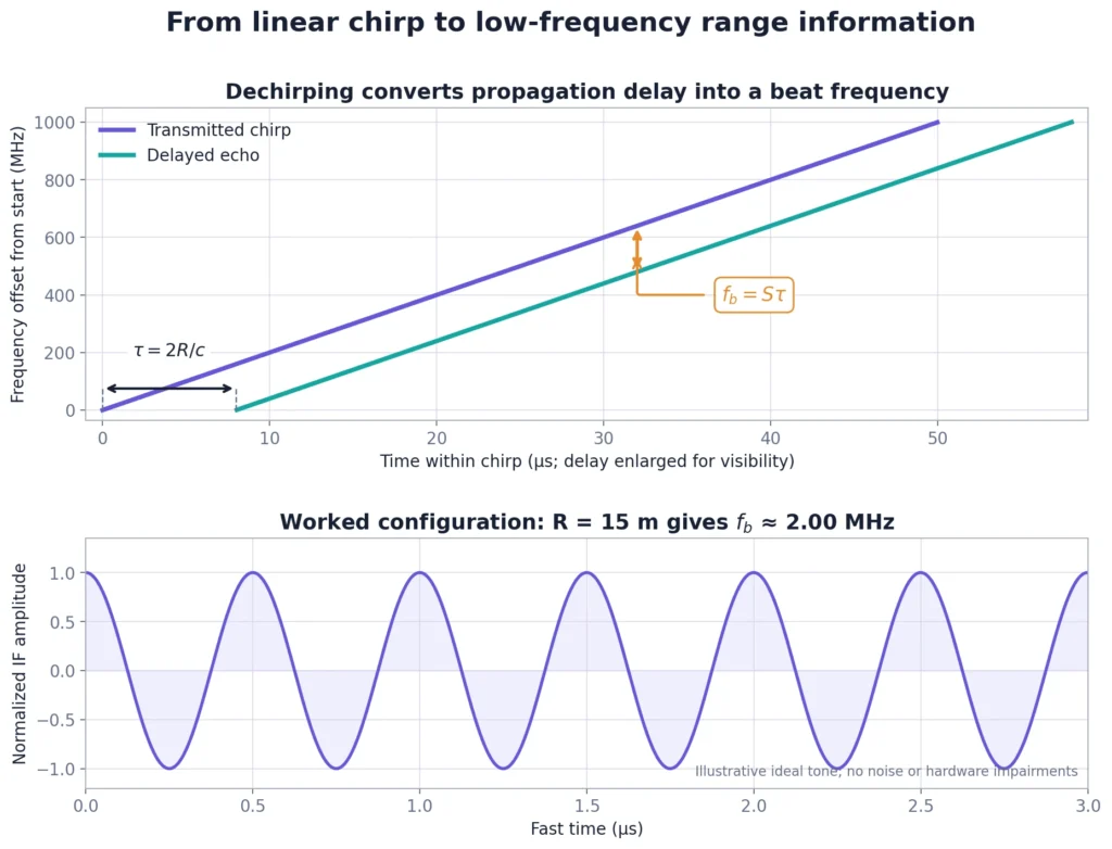
\tau=\frac{2R}{c},where c is propagation speed. Directly timing a delay of a few nanoseconds would be demanding. FMCW radar instead mixes, or dechirps, the received signal with a copy of the transmitted chirp. Using the product stx(t)srx*(t) as the sign convention, the stationary-target term is approximately
s_b(t)\approx\alpha\exp\!\left[j2\pi\left(S\tau t+f_c\tau-\frac{1}{2}S\tau^2\right)\right].The rapidly swept radio-frequency signal has become a much lower-frequency complex tone. Its beat frequency is proportional to delay:
f_b=S\tau=\frac{2SR}{c},\qquad R=\frac{cf_b}{2S}.This is the mathematical heart of FMCW ranging. The mixer has translated distance into a frequency that an ADC and FFT can estimate. The idea appears in early digital FM/CW treatments by Donald Barrick and in A. G. Stove’s later analysis of linear FMCW techniques.
For a moving target, Doppler also contributes to the within-chirp beat frequency, so a more honest first-order statement is
f_b\approx S\tau\mathbin{\pm}f_D.The sign depends on the mixer and velocity conventions. Fast-chirp processing commonly treats the delay term as dominant for the range FFT and estimates Doppler from the coherent phase progression across repeated chirps. This separation is approximate, not magical; high velocity, a shallow slope or a long ramp can produce noticeable range–Doppler coupling.
First dimension: the range FFT
Suppose the ADC collects N samples per chirp at sampling rate Fs, and a range FFT of length NR is used. For a positive beat-frequency convention, range bin k is mapped approximately by
f_b[k]=\frac{kF_s}{N_R},\qquad R[k]=\frac{c}{2S}\frac{kF_s}{N_R}.Each target contributes a complex sinusoid in fast time. Multiple ranges produce multiple tones, and the range FFT separates them to the degree allowed by the observed sweep bandwidth and window.
Range resolution is not the same as range-bin spacing
If the sampled portion of the chirp spans effective bandwidth Bobs, the familiar ideal resolution is
\Delta R_{\mathrm{resolution}}\approx\frac{c}{2B_{\mathrm{obs}}}.By contrast, the displayed FFT-grid spacing is
\Delta R_{\mathrm{bin}}=\frac{cF_s}{2SN_R}.When the FFT length equals the number of samples and the ADC observes the full linear sweep, these values coincide approximately. Zero-padding makes the grid denser, so a plotted peak can look smoother and its location can be interpolated more conveniently, but it does not create the bandwidth needed to resolve two closer targets.
| Range quantity | What it means | Main controls |
|---|---|---|
| Resolution | Ability to separate two nearby ideal targets | Observed sweep bandwidth and window |
| Bin spacing | Distance between samples on the plotted FFT grid | Sampling rate, slope and FFT length |
| Accuracy | Error in an estimated target range | SNR, calibration, chirp linearity, estimator, leakage and model error |
| Maximum usable range | Farthest range whose beat frequency and return strength remain usable | IF passband, ADC rate, slope, link budget and detection threshold |
If the usable analog and digital IF band ends at fIF,max, a frequency-limited boundary is
R_{\mathrm{IF}}\approx\frac{cf_{\mathrm{IF,max}}}{2S}.This is not a detection-range guarantee. A target inside that boundary can still be invisible because its return is too weak, masked by clutter or suppressed by filtering. Texas Instruments’ chirp-programming report treats IF bandwidth, sampling, sweep slope, timing, memory and SNR as coupled design constraints rather than independent specifications.
Second dimension: the Doppler FFT
A moving target changes range slightly between chirps. Even when that displacement is too small to move the range-FFT peak into a new bin, coherent phase is sensitive to it. For a monostatic radar, let positive v denote motion toward the radar. The Doppler frequency magnitude follows
f_D=\frac{2v}{\lambda},\qquad \lambda=\frac{c}{f_c}.If consecutive chirps begin Tc seconds apart, the phase increment at a target’s range bin is
\Delta\phi=2\pi f_DT_c=\frac{4\pi vT_c}{\lambda}.A Doppler FFT across M chirps separates different phase-increment rates. With uniformly spaced chirps, the ideal unambiguous velocity boundary and nominal Doppler-bin spacing are
|v|<v_{\max}=\frac{\lambda}{4T_c},\qquad \Delta v_{\mathrm{bin}}=\frac{\lambda}{2MT_c}.A shorter chirp repetition interval expands the unambiguous velocity interval. A longer coherent observation MTc produces finer Doppler spacing. Those goals compete with sweep bandwidth, idle time, maximum range, data transfer, frame rate and target stationarity. The TI fundamentals report derives the same relationships from the phase difference between chirps and explains why a second FFT is required when several targets share a range.
The Doppler FFT used for a single coherent frame should not be confused with a long-duration micro-Doppler spectrogram. The former estimates velocities across one coherent burst; the latter uses a sequence of windows to reveal how Doppler content changes over time. For that next layer, see ArthaVedya’s guide to choosing STFT parameters for radar micro-Doppler.
Third dimension: the angle FFT
Range and velocity cannot separate two targets that occupy the same range–Doppler cell. An array can separate them when their waves arrive from different directions.
For an ideal uniform linear array with element spacing d, a far-field plane wave arriving at angle θ produces an inter-element phase increment
\psi=\frac{2\pi d}{\lambda}\sin\theta.Once that phase slope is estimated, angle follows from
\theta=\sin^{-1}\!\left(\frac{\lambda\psi}{2\pi d}\right).An angle FFT is therefore a spatial-frequency estimator. Its bins are uniform in u = sin θ, not in degrees. For a centered FFT index ℓ and transform length NA,
u[\ell]=\sin\theta[\ell]=\frac{\lambda}{d}\frac{\ell}{N_A}.Plotting FFT index linearly as angle is wrong except as a small-angle approximation. Each spatial bin must first be mapped to sin θ and then through the inverse sine. Spacing d = λ/2 gives the widest ideal unambiguous field of view for a simple uniform array, although the real antenna pattern may provide much less useful coverage.
Near boresight, an unwindowed array of P half-wavelength-spaced elements has spatial FFT-bin spacing of roughly 2/P radians. This is only a first-order resolution guide. Aperture geometry, tapering, SNR, correlated reflections and the estimator all matter, and zero-padding the angle FFT cannot enlarge the physical aperture.
Physical and virtual antennas
MIMO radar can synthesize more spatial samples from multiple transmit and receive antennas. With suitable placement, NTX transmitters and NRX receivers can form as many as NTXNRX virtual positions. They do not automatically behave like simultaneous, perfectly calibrated physical sensors.
In time-division-multiplexed MIMO, different transmitters illuminate the scene at different instants. Target motion then introduces transmitter-dependent phase that can bias the angle estimate unless it is compensated. Sandeep Rao’s official MIMO radar application report explicitly places Doppler correction before the angle FFT in this workflow.
One point-target model unifies all three dimensions
Under an ideal narrowband-array, fast-chirp approximation, and assuming each target’s range, velocity and angle remain effectively constant during one coherent processing interval, the sampled cube can be written as
x[n,m,p]\approx\sum_{i=1}^{K}\alpha_i\exp\!\left\{j2\pi\left(\frac{f_{b,i}}{F_s}n+f_{D,i}T_cm+\frac{d\sin\theta_i}{\lambda}p\right)\right\}+w[n,m,p].For each point target, the phase is approximately linear along all three axes. The coefficient of n carries range, the coefficient of m carries Doppler, and the coefficient of p carries angle. Noise is represented by w[n,m,p]. This equation is the compact reason multidimensional Fourier processing works.
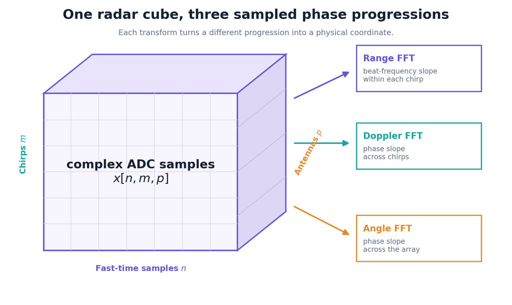
Figure 2. An FMCW radar cube contains three sampled phase progressions: fast time for range, slow time for Doppler and array position for angle.With separate windows along the three dimensions, a conceptual 3-D transform is
X[k,q,\ell]=\sum_n\sum_m\sum_p x[n,m,p]w_R[n]w_D[m]w_A[p]\exp\!\left[-j2\pi\left(\frac{kn}{N_R}+\frac{qm}{N_D}+\frac{\ell p}{N_A}\right)\right].A full 3-D FFT is not always the efficient implementation. Many real systems first form range–Doppler matrices, combine power across channels for detection, and calculate angle only at detected range–Doppler cells. That avoids constructing a dense angle spectrum where no target was detected.
A worked 77 GHz example
Consider an illustrative, idealized FMCW configuration. These are design values for explaining the mathematics, not the specification of a particular radar chip.
| Parameter | Value | Role |
|---|---|---|
| Carrier frequency | 77 GHz | Sets wavelength and Doppler scale |
| Sweep bandwidth | 1 GHz | Sets ideal range resolution |
| Ramp time | 50 µs | With bandwidth, gives slope |
| Idle time | 10 µs | Makes chirp repetition interval 60 µs |
| ADC rate | 10 MS/s complex | 500 samples during each ramp |
| Chirps per coherent frame | 128 | Gives a 7.68 ms active coherent interval |
| Array | 12 ideal elements at λ/2 spacing | Provides the sampled angle aperture |
The wavelength and slope are 3.893 mm and 20 MHz/µs, respectively. The resulting first-order limits are:
- Ideal range resolution: 0.150 m from c/(2B).
- Frequency-limited range in this simulation: 37.47 m when the usable positive beat-frequency boundary is assumed to be Fs/2. A real device’s usable IF passband must replace that assumption.
- Unambiguous radial-speed magnitude: 16.22 m/s, or about 58.4 km/h, from λ/(4Tc).
- Nominal Doppler-bin spacing: 0.253 m/s from λ/(2MTc).
- Unwindowed spatial-bin spacing near boresight: about 9.6° for 12 half-wavelength-spaced elements. This is not a universal angle-accuracy claim.
The accompanying point-target simulation uses four reflectors:
| Target | Range | Radial velocity | Angle | Purpose in the example |
|---|---|---|---|---|
| A | 8.10 m | +2.00 m/s | −25° | Separate in range and Doppler |
| B | 16.50 m | −3.00 m/s | +8° | Shares range and velocity with C |
| C | 16.50 m | −3.00 m/s | +32° | Requires the angle dimension to separate from B |
| D | 16.50 m | +1.00 m/s | −6° | Shares range with B and C but separates in Doppler |
The range–Doppler map shows A and D as separate peaks. B and C deliberately collapse into one range–Doppler cell because their range and velocity are identical. The angle spectrum evaluated at that cell resolves two directions near 8° and 32°. This is precisely what the third dimension contributes.
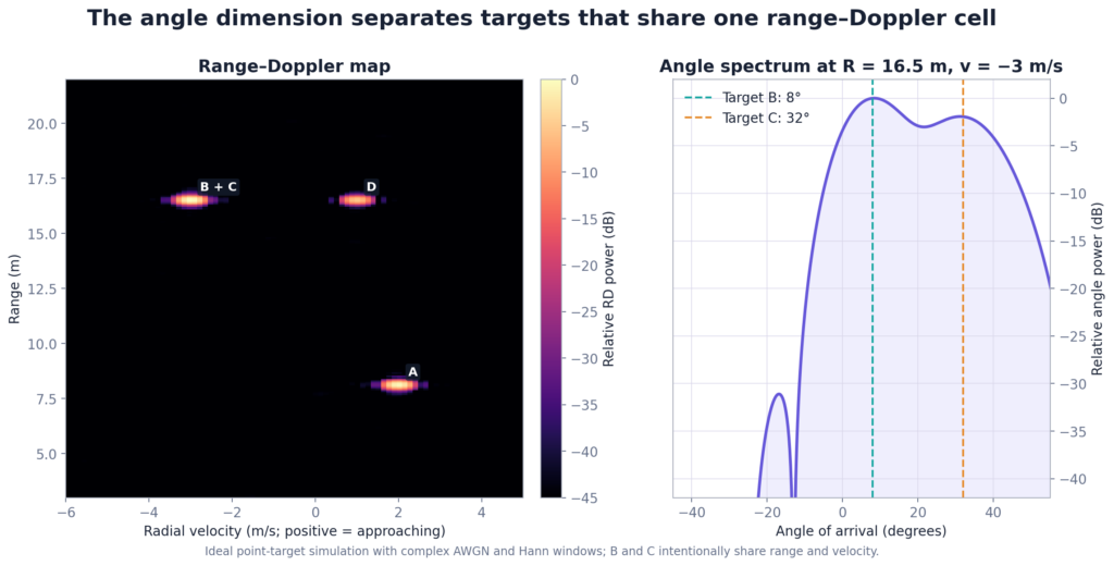
The figure is an original simulation, not measured radar data. It uses the separable point-target equation above, complex additive white Gaussian noise and Hann windows. It intentionally omits antenna-pattern variation, multipath, phase noise, chirp nonlinearity, mutual coupling, target extent, range migration and TDM timing. Those omissions make the three dimensions interpretable; they also limit what the result can prove.
The processing chain in compact form
A practical baseline can be expressed without hiding the dimensions:
input: complex cube x[fast_time, chirp, antenna]

for every chirp and antenna:
    range_spectrum = FFT(window_range * x, axis=fast_time)

for every range bin and antenna:
    range_doppler = FFTshift(FFT(window_doppler * range_spectrum,
                                 axis=chirp))

predetection_power = sum(abs(range_doppler)**2, axis=antenna)
detections = CFAR_or_other_detector(predetection_power)

for each detected range–Doppler cell:
    calibrated_spatial_vector = range_doppler[cell, :]
    angle_spectrum = FFTshift(FFT(window_angle * calibrated_spatial_vector))
    map spatial frequency to sin(theta), then to theta
The order communicates an important distinction: an FFT produces spectral estimates; it does not decide which cells are targets. Detection is a separate statistical problem. Constant-false-alarm-rate methods estimate a local background and adapt the threshold, but their behaviour depends on clutter, interfering targets, guard cells and training cells. Hermann Rohling’s foundational CFAR analysis remains useful precisely because “bright” and “detected” are not equivalent.
How the main design parameters trade against one another
| If you increase… | Primary benefit | What you may pay |
|---|---|---|
| Sweep bandwidth B | Finer range resolution | More demanding RF linearity, regulation and possibly sampling/IF requirements |
| Chirp slope S | Larger beat separation for a given range difference; same bandwidth in less time | Higher beat frequency at a given range and wider required IF bandwidth |
| ADC rate or usable IF bandwidth | Larger frequency-limited range for fixed slope | More data, memory, interface bandwidth and processing |
| Chirps per coherent interval M | Finer Doppler spacing and coherent gain | Longer latency, more data and greater risk of target nonstationarity |
| Chirp repetition frequency | Larger unambiguous Doppler interval | Less time for ramp, idle, settling and data movement |
| Physical array aperture | Finer angular resolution | Larger hardware, calibration burden and possible grating-lobe constraints |
| FFT zero-padding | Denser plotted grid and easier peak interpolation | More computation; no new physical resolution |
| Window sidelobe suppression | Less leakage from strong targets | Wider mainlobe and reduced ability to separate close targets |
No single chirp setting maximizes all useful properties. The radar-design task is to choose a feasible point in this coupled space. The broad comparison of 24, 60 and 77 GHz radar for human sensing explains why carrier frequency alone cannot choose the best sensor: available bandwidth, aperture, regulations, link budget and raw-data access also matter.
Design backwards from the measurement requirement
A defensible configuration begins with the scene and required separation, not with an arbitrary FFT size.
- Set range resolution from the closest targets that must be separated. If 0.10 m ideal resolution is required, the observed bandwidth must satisfy Bobs ≥ c/(2 × 0.10 m), or about 1.50 GHz.
- Set unambiguous velocity from the fastest expected radial motion. Choose the effective slow-time interval so that λ/(4Tc,eff) exceeds that speed with margin.
- Set coherent duration from the velocity separation requirement. Choose MTc,eff to reach the desired Doppler spacing while keeping target motion sufficiently stable.
- Choose slope, ADC rate and IF passband together. Verify that the maximum range maps inside the usable beat-frequency band, including Doppler and filter margins.
- Choose aperture from angular separation, not angle-FFT length. Then check field of view, grating lobes, antenna gain and calibration.
- Budget the complete cube. The worked example contains 500 × 128 × 12 = 768,000 complex samples per frame. Stored as complex float32, that is about 6.14 MB before metadata or intermediate arrays.
- Validate with controlled targets. Test known ranges, approach and departure, two-target separation, broadside and off-axis angles, and stationary clutter before interpreting complex scenes.
This reverse-design approach follows the engineering logic in the application reports above and in the broader signal-processing review by Patole and colleagues (2017): range, Doppler, angle, waveform timing, detection and hardware limits belong to one chain.
Eleven mistakes that produce convincing but wrong maps
- Using ramp time where chirp repetition interval is required. Doppler sampling depends on the time between corresponding chirps, including idle time and multiplexing.
- Using ADC rate as slow-time sampling rate. The ADC rate defines fast-time sampling; chirp timing defines ordinary Doppler sampling.
- Discarding complex phase too early. Magnitude-only range profiles cannot preserve the phase progression needed for signed Doppler and angle.
- Calling zero-padded bins “resolution.” A longer FFT interpolates the spectrum but does not add bandwidth, coherent time or aperture.
- Plotting angle bins linearly in degrees. A uniform linear array samples sin θ; the inverse-sine mapping is nonlinear.
- Ignoring channel calibration. Cable, RF-chain and antenna phase errors can look like target angle.
- Ignoring TDM-MIMO motion phase. Sequential transmitter timing can mix Doppler into the virtual-array phase.
- Assuming one peak equals one physical object. Several scatterers can occupy one cell, while one extended object can occupy many cells.
- Reading colour as radar cross section without calibration. Window gain, range loss, antenna gain, automatic gain control and display normalization alter intensity.
- Ignoring range–Doppler coupling and migration. Fast targets can shift apparent range or move across bins during a coherent interval.
- Tuning only for a pretty heatmap. Clipping, smoothing and aggressive background removal can conceal sidelobes, slow targets and failure modes.
From radar maps to human sensing and machine learning
For human sensing, a range–Doppler–angle frame is usually an intermediate representation rather than the final answer. Range can isolate a person from background reflectors, Doppler captures radial body motion, and angle helps separate directions or people. Across time, sequences of maps reveal motion dynamics.
Fine articulation can also spread energy around the bulk body return. ArthaVedya’s guide to how radar sees arms, legs and human motion explains why those patterns represent superposed radial velocities rather than literal limb images. Google Soli pushed the same principle toward small hand movements; our Soli paper breakdown separates its controlled experimental result from stronger claims it did not establish.
Machine-learning performance still depends on the measurement chain. A network cannot repair mislabeled axes, aliased velocity, leaked train–test recordings or a deployment geometry absent from training. The practical guide to starting radar-based human activity recognition research covers those dataset and evaluation decisions.
Key takeaways
- FMCW dechirping converts round-trip delay into a beat frequency that can be mapped to range.
- The range FFT acts within each chirp; the Doppler FFT acts across coherent chirps; the angle FFT or beamformer acts across calibrated antenna channels.
- Range, Doppler and angle are three estimates of phase progression along different axes of one complex radar cube.
- Bandwidth controls ideal range resolution, coherent duration controls Doppler spacing, and physical aperture controls angular resolution.
- FFT length controls grid density; it does not independently create physical resolution.
- A map is not a detection list or an image of object shape. Windowing, calibration, CFAR, clustering and tracking answer different questions.
- TDM-MIMO timing, chirp nonlinearity, coupling, multipath and target motion can break the ideal separable model and must be tested on real hardware.
The most reliable mental model is also the simplest: preserve the complex cube, identify what is being sampled along each axis, transform the correct dimension, and calibrate every spectral bin back to physics. Once those steps are explicit, a range–Doppler–angle map stops being a colourful black box and becomes a measurable engineering object.
Simulation note: All figures are original simulations based on an ideal FMCW point-target model with seeded noise. They use no measured radar data and exclude real-world hardware and propagation impairments.
References
- D. E. Barrick, “FM/CW Radar Signals and Digital Processing,” NOAA Technical Report ERL 283-WPL 26, 1973.
- A. G. Stove, “Linear FMCW Radar Techniques,” IEE Proceedings F—Radar and Signal Processing, vol. 139, no. 5, pp. 343–350, 1992. DOI: 10.1049/ip-f-2.1992.0048.
- C. Iovescu and S. Rao, “The Fundamentals of Millimeter Wave Radar Sensors,” Texas Instruments, revised 2020.
- V. Dham, “Programming Chirp Parameters in TI Radar Devices,” Texas Instruments Application Report SWRA553A, revised 2020.
- S. Rao, “MIMO Radar,” Texas Instruments Application Report SWRA554A, revised 2018.
- S. M. Patole, M. Torlak, D. Wang and M. Ali, “Automotive Radars: A Review of Signal Processing Techniques,” IEEE Signal Processing Magazine, vol. 34, no. 2, pp. 22–35, 2017. DOI: 10.1109/MSP.2016.2628914.
- H. Rohling, “Radar CFAR Thresholding in Clutter and Multiple Target Situations,” IEEE Transactions on Aerospace and Electronic Systems, vol. AES-19, no. 4, pp. 608–621, 1983. DOI: 10.1109/TAES.1983.309350.
- Infineon Technologies, “FMCW Radar Digital Signal Processing,” training handout, 2022.