CFAR is a family of adaptive threshold detectors, not one algorithm. Choose CA-CFAR for a reasonably homogeneous background with isolated targets. Choose GO-CFAR when an abrupt clutter increase makes false-alarm control the priority. Consider SO-CFAR when one reference half may be contaminated but the other is plausibly representative. Choose OS-CFAR when several large training-cell outliers or nearby targets are expected and the implementation can support sorting or selection.
That rule is only a starting point. The decision also depends on which quantity enters the detector, how many cells a target occupies, the geometry of the training window and what “false alarm” means for the complete radar pipeline. Most importantly, CA, GO, SO and OS must use different threshold factors when they are compared at the same nominal false-alarm probability.
Short answer: begin with CA-CFAR as the homogeneous-background baseline. Add GO-CFAR if clutter-edge false alarms dominate, or OS-CFAR if neighbouring targets cause masking. Use SO-CFAR deliberately, not as a generally “more sensitive” option, because its quieter-side estimate can become dangerously low on the high-clutter side of an edge. Calibrate every method separately and verify the achieved false-alarm rate on target-free data.
The fastest defensible choice
| Local situation | Strong first choice | Why | Main check before deployment |
|---|---|---|---|
| Homogeneous noise or clutter; isolated targets | CA-CFAR | Uses all training cells efficiently and is simple to implement | Are the training samples sufficiently representative and weakly correlated? |
| Window straddles an abrupt rise in clutter | GO-CFAR | Uses the louder half and resists underestimating the high-clutter side | Can the resulting conservative threshold hide a target on the quiet side? |
| One half contains a strong neighbour; the other half is clean | SO-CFAR or OS-CFAR | SO can select the clean half; OS can reject a limited number of large cells | Is the quiet half truly representative, and how many cells are contaminated? |
| Several nearby targets or sparse high outliers | OS-CFAR | A selected order statistic is not pulled upward by every large sample | Does the chosen rank tolerate the expected number and width of interferers? |
| Structured, heavy-tailed or poorly modelled background | No classical variant is automatically safe | The nominal CFAR model may not describe the data | Calibrate and report performance on representative target-free measurements |
This article uses GO-CFAR and SO-CFAR as readable names. Software and hardware documentation may instead use GOCA, SOCA, CAGO or CASO. The operations are what matter: greatest-of chooses the larger of two half-window averages, and smallest-of chooses the smaller. The current MATLAB detector documentation, for example, uses the labels CA, GOCA, SOCA and OS for these four estimators (MathWorks, CFARDetector).
What CFAR makes constant—and what it does not
A fixed threshold behaves poorly when receiver noise, interference or clutter power changes across range, Doppler, angle or time. CFAR replaces that fixed level with a local estimate. For each cell under test (CUT), it measures surrounding reference cells, multiplies the resulting statistic by a scale factor and declares a detection if the CUT exceeds the threshold.
T=\alpha Z,\qquad \text{detect if }x_{\mathrm{CUT}}>T.Here, Z is a local background statistic and α is a method-specific threshold factor. The name “constant false alarm rate” does not mean that a deployed detector produces exactly the requested rate everywhere. It means that, under a stated statistical model and correct calibration, scaling all background powers by the same amount does not change the nominal probability that a target-free CUT crosses the threshold. Nonhomogeneous clutter, correlated bins, interference, pulse integration and an incorrect input domain can all break that promise. Classical analyses of these failures include Gandhi and Kassam (1988).
PFA is normally a per-CUT probability
A configured false-alarm probability of 10−4 is not automatically “one false object in 10,000 frames.” It is usually a probability for one tested cell under the assumed target-free model. If a frame tests M cells and each has nominal probability PFA, the expected number of false cells is
\mathbb{E}[N_{\mathrm{FA}}]=M P_{\mathrm{FA}}.A 256 × 64 range–Doppler search region contains 16,384 CUTs. At PFA = 10−4, the nominal expectation is therefore 1.64 false cells per frame, or about 32.8 false cells per second at 20 frames/s. Correlation changes the clustering and variability of those events, while nonhomogeneity changes the rate itself. Peak grouping, clustering and tracking can reduce the number of false objects, but they do not change what the original per-cell setting meant.
One sliding window, four background estimators
A conventional one-dimensional CFAR window contains leading training cells, guard cells, the CUT, another guard band and lagging training cells. Training cells estimate the local background. Guard cells prevent the target’s mainlobe, sidelobes or spatial extent from contaminating that estimate. The complete window slides so that each eligible bin becomes the CUT in turn.
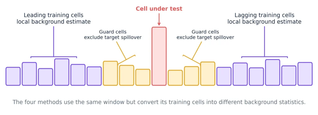
Let there be N training powers in total and equal half-windows with means ZL and ZR. CA-CFAR averages every training cell:
Z_{\mathrm{CA}}=\frac{1}{N}\sum_{i=1}^{N}x_i.GO-CFAR and SO-CFAR split the same training region and then make opposite choices:
Z_{\mathrm{GO}}=\max(Z_L,Z_R),\qquad Z_{\mathrm{SO}}=\min(Z_L,Z_R).OS-CFAR sorts all training powers in ascending order and selects the kth:
x_{(1)}\le x_{(2)}\le\cdots\le x_{(N)},\qquad Z_{\mathrm{OS}}=x_{(k)}.The window is shared; the assumed background evidence is not. CA trusts every training cell. GO trusts the louder side. SO trusts the quieter side. OS trusts a selected quantile. Those four choices explain nearly all of their characteristic successes and failures.
CA-CFAR: the baseline for homogeneous backgrounds
CA-CFAR pools all training powers into one mean. When those cells are independent samples from the same background distribution and no target leaks into them, averaging produces a stable estimate with low computational cost. It is therefore the correct first baseline for most new implementations—not because it is universally best, but because every more robust method should justify the sensitivity or complexity it trades away.
For independent exponential training powers—the square-law output produced by circular complex Gaussian noise—with one noncoherently processed sample per cell, the CA threshold factor for N total training cells is
\alpha_{\mathrm{CA}}=N\left(P_{\mathrm{FA}}^{-1/N}-1\right).The derivation and assumptions are also documented in the official MathWorks CFAR example. The formula is compact, but its scope is narrow: it is not automatically valid for magnitude data, averaged decibels, correlated bins, noncoherent integration of several pulses or arbitrary clutter distributions.
Where CA fails
- A neighbouring target enters the training window. Its large power raises the mean, which can hide the CUT target. This is target masking.
- The window straddles a clutter edge. On the high-clutter side, low-power training cells from the quiet region can pull the estimate down and create excessive false alarms. On the quiet side, high-clutter cells can push it up and reduce detection probability.
- The background has sparse large outliers. An arithmetic mean gives every outlier unbounded influence.
Increasing the number of training cells reduces random variation in a homogeneous estimate, but it also makes the window physically wider and more likely to cross a boundary or include another target. More training cells are not unconditionally better.
GO-CFAR: conservative protection at clutter edges
GO-CFAR averages the leading and lagging halves separately and uses the larger mean. The logic was developed to improve behaviour when the reference window crosses an abrupt change in clutter level; the classical detectability cost of greatest-of selection in homogeneous conditions was analysed by Hansen and Sawyers (1980).
Suppose the CUT has just entered a high-clutter region while one training half still lies in quiet background. CA blends the two levels and can underestimate the local high background. GO chooses the high-side mean, raises the threshold and suppresses the burst of false alarms that would otherwise appear along the boundary.
The same conservatism creates GO’s main costs. If the CUT is on the quiet side of the edge, the louder half can set an unnecessarily high threshold. A strong neighbouring target in only one training half is also likely to make that half the maximum, so GO can worsen target masking. It is best viewed as an edge-protection rule, not as a general multiple-target solution.
SO-CFAR: useful when one side is clean—and risky when it is not
SO-CFAR chooses the smaller of the two half-window means. If a strong neighbouring target contaminates only the leading half, SO can ignore that half and retain a threshold based on the clean lagging side. This can preserve a weaker CUT that CA or GO would mask.
But the word “smaller” should trigger caution. When the CUT is in a high-clutter region and the opposite half-window still sees quiet background, SO selects the quiet side. The resulting threshold can be far below the CUT’s true local background and generate a line of false alarms. If both halves contain nearby targets, SO also loses its one-clean-side advantage.
SO-CFAR is therefore appropriate only when the scene or processing geometry gives a credible reason to trust the quieter reference half. Its apparent sensitivity is not free; it is purchased with weaker protection against upward clutter transitions.
OS-CFAR: robustness through a chosen rank
OS-CFAR replaces averaging with sorting. After arranging the N training powers from smallest to largest, it selects the kth value. A few very large cells can then sit above the chosen rank without directly changing the background statistic. Rohling’s foundational study proposed this approach for clutter edges and multiple-target situations (Rohling, 1983), with later theory examining nonuniform clutter and multiple targets in more detail (Blake, 1988).
With ascending one-based indexing, up to N − k sufficiently large contaminated cells can remain above the selected value. For N = 32 and k = 24, that simple count is eight. It is a design intuition, not a guarantee: wide targets, moderate contaminants, mixed clutter populations and correlation can still shift the order statistic.
Under the same independent exponential-power model, the nominal OS false-alarm probability satisfies
P_{\mathrm{FA,OS}}=\prod_{i=0}^{k-1}\frac{N-i}{N-i+\alpha_{\mathrm{OS}}}.The factor αOS is normally solved numerically for the chosen N, k and PFA. Rank conventions are a common source of silent errors: “rank 24” may mean the 24th smallest value in one library, a zero-based array position in another or occasionally a rank counted from the largest end. State the ordering and indexing explicitly.
Rohling found a rank around three quarters of the reference cells useful in the studied model, and k ≈ 0.75N remains a common starting point. It is not a universal optimum. Rank and threshold factor form a pair: changing k without recalibrating α changes the false-alarm rate as well as the robustness.
The comparison most implementations get wrong: equal PFA first
It is tempting to calculate CA-CFAR’s multiplier once and reuse it for GO, SO and OS because every method eventually computes T = αZ. That does not create a fair experiment. The four estimators have different probability distributions, so the same α produces four different nominal false-alarm probabilities.
Consider 32 independent exponential training powers, 16 on each side, a target PFA of 10−4 and OS rank k = 24. Using half-window means for GO and SO and the 24th-smallest raw power for OS gives the following exact numerical calibration:
| Method | Correct α for nominal PFA = 10−4 | Nominal PFA if CA’s α = 10.6727 is reused | Error relative to target |
|---|---|---|---|
| CA | 10.6727 | 1.000 × 10⁻⁴ | 1.00× |
| GO | 9.6307 | 4.320 × 10⁻⁵ | 0.43× |
| SO | 13.6305 | 5.190 × 10⁻⁴ | 5.19× |
| OS, k = 24 | 8.5801 | 1.711 × 10⁻⁵ | 0.17× |
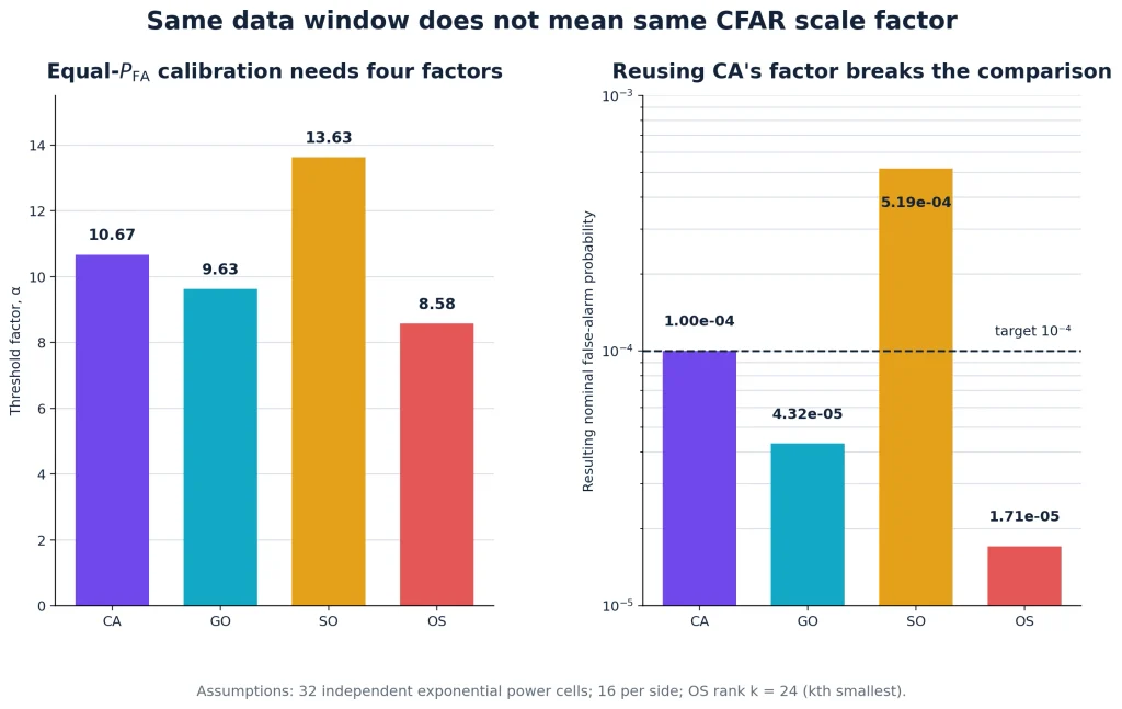
Reusing CA’s factor would make SO appear more sensitive partly because it is allowed about 5.2 times the intended false-alarm probability. GO and OS would appear more conservative partly because their actual nominal rates would be lower than requested. Detection probability, CFAR loss and robustness should be compared only after each method has been calibrated to the same PFA.
The raw α values are not a performance ranking either. OS selects a relatively high raw cell rather than an average, while SO selects a relatively low half mean; their multipliers compensate for differently distributed statistics. Compare achieved false alarms and detection probability, not multiplier magnitude.
How the four methods behave in the scenes that matter
1. Homogeneous background with an isolated target
CA is the natural baseline because all training cells are valid evidence from one background population. GO and SO discard part of the symmetry by selecting one half, while OS reduces the data to one rank. At equal PFA, those robustness choices generally impose some detectability cost in the ideal scene they were not designed to fix. Start with CA here and demand evidence before adding complexity.
2. A clutter edge passes through the reference window
There are two sides to the same edge. When the CUT lies just inside the high-power region, CA may average high and low references and set the threshold too low; GO protects this side by following the larger half. When the CUT lies on the low-power side, GO may overestimate its background and miss a target. SO exhibits the opposite bias. OS changes behaviour when enough high-clutter cells cross its chosen rank, so it can handle some edges well but is not direction-free or rank-free.
3. A strong secondary target enters one training half
CA’s mean rises. GO is likely to select the contaminated half and can rise even more. SO can select the clean half, while OS can leave a limited number of large target cells above its rank. If the interfering return spreads across both halves, SO no longer has a clean reference and OS robustness depends on the contaminated-cell count relative to N − k.
4. Extended objects or dense target groups occupy many cells
No classical variant can manufacture clean training data. A human, vehicle or target sidelobe pattern may occupy several adjacent range–Doppler cells, and several objects may contaminate both sides. Increase the guard region to cover predictable target spillover, use OS only with a rank justified by the maximum expected occupancy, or incorporate censoring, clutter maps, segmentation or track-level logic. Calling OS “robust to multiple targets” without stating target width and rank is incomplete.
Choose training cells, guard cells and rank in physical units
A parameter such as “four guard cells” has no portable physical meaning. It depends on range-bin spacing, Doppler-bin spacing, FFT windowing, zero-padding and the target’s expected extent. The range–Doppler–angle mathematics guide explains how those axes and bin spacings are formed.
- Define counts unambiguously. State whether training and guard counts are totals or per-side values. For example, MATLAB’s one-dimensional object defines an even total count split across both sides, while many handwritten implementations specify a count per side.
- Size the guard region from target leakage. Inspect the processed point-spread function with the actual range and Doppler windows. Include the mainlobe, significant sidelobes and expected object extent. Zero-padding creates more plotted bins without improving physical resolution, so the guard-cell count may need to increase merely to preserve the same exclusion width.
- Keep the training region locally stationary. More cells reduce estimator variance in a homogeneous background, but a wider span crosses more clutter boundaries and contains more neighbours. Tune the physical span, not only the integer count.
- Treat OS rank and α as one configuration. Choose the number of high cells the detector should tolerate, convert that requirement into a candidate rank and then recalibrate the multiplier for that exact rank.
- Choose PFA from a system budget. Work backward from acceptable false cells per frame, then from false clusters or tracks per minute. A copied value such as 10−3 or 10−5 is not a design justification.
Range–Doppler CFAR is not simply one-dimensional CFAR run twice
On a range–Doppler map, the CUT has a two-dimensional guard region and a surrounding training region. Their shape encodes assumptions: range sidelobes and object length need not match Doppler broadening, and the zero-Doppler clutter ridge may be highly anisotropic. A rectangular ring, cross-shaped stencil and separate range-then-Doppler tests therefore use different reference evidence and need separate validation.
Edge handling matters too. Range is normally bounded, so wrapping the farthest range bins into the nearest bins would mix unrelated cells. The Doppler FFT grid is cyclic, so circular indexing can sometimes be appropriate near the unambiguous-velocity boundary. Skipping incomplete CUTs is often safer than padding missing training cells with zeros, which biases the estimate downward. If a window is shrunk at an edge, its threshold factor must be recalibrated for the changed sample count.
A CFAR pass produces detected cells, not objects. Local-maximum tests, peak grouping, connected components, clustering, angle estimation and tracking determine what becomes a report. Texas Instruments’ radar hardware accelerator guide, for example, documents CA, CAGO and CASO modes, optional local-maximum grouping and different linear/log input paths; it also states that OS is not supported by that particular engine (TI SWRU527A). This is a useful reminder that the statistically preferred method and the available hardware method may differ.
For the surrounding implementation context, see the end-to-end guide from raw ADC samples to activity labels. The distinction also changes how public data can be used: a released point cloud has normally already passed through device-specific detection and thresholding, so it cannot support a new ADC- or CFAR-level contribution. Our radar-HAR dataset comparison separates those representation levels.
Power, magnitude and decibels change the threshold mathematics
The closed-form CA multiplier above assumes exponential power samples. Complex Gaussian I/Q passed through a square-law detector gives that distribution for a single look. Magnitude follows a Rayleigh distribution instead. A sum of several noncoherently integrated powers follows another distribution, and windowed FFT bins are often correlated. Feeding any of these into the same formula without adjustment does not preserve the requested PFA.
Decibel processing creates another trap. If ZdB is obtained by converting the same linear-power statistic Z to decibels, multiplication becomes addition:
T_{\mathrm{dB}}=Z_{\mathrm{dB}}+10\log_{10}\alpha.But averaging individual dB-valued training cells and then adding 10 log10 α is not equivalent to averaging linear powers and converting the result. The logarithm and arithmetic mean do not commute. Document whether the detector receives complex samples, magnitude, power, log magnitude or log power, and reproduce the exact quantization and averaging used by the target hardware.
A minimal implementation skeleton
for each valid CUT:
    left  = leading training powers
    right = lagging training powers
    train = concatenate(left, right)

    if method == "CA": z = mean(train)
    if method == "GO": z = max(mean(left), mean(right))
    if method == "SO": z = min(mean(left), mean(right))
    if method == "OS": z = kth_smallest(train, k)

    threshold = alpha[method, N, k, input_model] * z
    detection = power[CUT] > threshold
The important line is the indexed α. It must correspond to the estimator, number of training cells, OS rank where applicable, detector input distribution and integration model. After this cell-level test, apply separately documented peak grouping and object-level filtering.
A validation protocol that can support a research claim
- Freeze the data contract. Record the input domain, normalization, integration, FFT windows, bin spacing, training and guard counts, edge rule, OS ordering and rank convention.
- Calibrate each method independently. Use the correct analytic relation where the assumptions hold; otherwise solve α using Monte Carlo or representative calibration data.
- Verify the ideal case. Generate target-free data from the stated model, disable peak grouping and confirm the empirical per-CUT false-alarm rate with uncertainty bounds.
- Measure real target-free backgrounds. Include different ranges, Doppler regions, rooms, weather or operating modes. Report where the achieved rate departs from the nominal value instead of averaging every regime into one number.
- Test clutter edges in both directions. Evaluate CUTs on the quiet and loud sides separately; a method can solve one side while worsening the other.
- Sweep interference structure. Vary neighbour power, distance from the CUT, occupied-cell width and whether contaminants appear on one or both sides.
- Measure detection probability at equal achieved PFA. Compare PD versus SNR or signal-to-clutter ratio only after the false-alarm operating points are matched.
- Report two output levels. Give false cells per tested cell and per frame before grouping, then false clusters or tracks per unit time after the complete pipeline.
A single attractive range–Doppler screenshot is not a detector evaluation. At minimum, publish the parameter table, achieved false-alarm rates, detection curves and the nonhomogeneous cases that motivated the selected variant.
Common CFAR mistakes
- Calling PFA a per-frame probability without accounting for the number of tested cells.
- Reusing one threshold multiplier across CA, GO, SO and OS.
- Applying a square-law power formula to magnitude or dB samples.
- Reporting “32 training cells” without saying total or per side.
- Choosing guard cells by habit rather than the measured target response and physical bin widths.
- Padding missing edge references with zeros, which lowers the estimated background.
- Assuming OS handles any number of targets without relating contaminated-cell count to N − k.
- Forcing a top-K output when no cell passes CFAR. That converts a valid empty detection set into fabricated objects.
- Comparing only detection counts. More detections can mean higher PD, higher PFA or both.
What we would use first
For a new FMCW radar project, we would implement and validate CA-CFAR first. It creates a transparent baseline and exposes whether the background is actually homogeneous. We would then add one alternative tied to an observed failure: GO if clutter-edge false alarms dominate, or OS if neighbouring detections raise the reference estimate and mask weaker targets.
We would use SO only when measurements show that one side is often clean and the cost of high-side edge false alarms is controlled elsewhere. If scene classification or switching logic selects methods dynamically, each branch and the switching boundary must be calibrated; “adaptive CFAR” does not inherit a constant false-alarm rate merely by choosing among algorithms.
The final choice should be made with a small stress-test matrix, not a slogan: homogeneous background, upward and downward clutter edges, one-sided and two-sided interferers, extended targets, real target-free data and the full grouping/tracking chain. The best detector is the simplest one that meets the system’s detection and false-report budgets across those conditions.
Key takeaways
- CA, GO, SO and OS use different local background statistics; CFAR is not one interchangeable algorithm.
- CA is the strongest baseline for homogeneous backgrounds, GO protects the high side of clutter edges, SO can exploit one clean half and OS can tolerate a limited number of large training cells.
- Every method requires its own threshold factor at a common nominal PFA. Reusing CA’s multiplier can reverse the apparent comparison.
- A configured PFA is normally per tested cell. Convert it into expected false cells per frame and then measure false objects after grouping and tracking.
- Training, guard and OS-rank settings must be tied to physical target width, clutter stationarity and expected contaminant occupancy.
- The input domain matters. Power, magnitude, integrated power and decibels require different threshold mathematics or empirical calibration.
- No classical CFAR variant guarantees a constant rate in arbitrary real clutter. Validate on target-free measurements and stress the failure mode that motivated the algorithm.
References
- Finn, H. M., & Johnson, R. S. (1968). Adaptive Detection Mode with Threshold Control as a Function of Spatially Sampled Clutter-Level Estimates. RCA Review, 29(3), 414–464.
- Hansen, V. G., & Sawyers, J. H. (1980). Detectability Loss Due to “Greatest Of” Selection in a Cell-Averaging CFAR. IEEE Transactions on Aerospace and Electronic Systems, AES-16(1), 115–118.
- Rohling, H. (1983). Radar CFAR Thresholding in Clutter and Multiple Target Situations. IEEE Transactions on Aerospace and Electronic Systems, AES-19(4), 608–621.
- Gandhi, P. P., & Kassam, S. A. (1988). Analysis of CFAR Processors in Nonhomogeneous Background. IEEE Transactions on Aerospace and Electronic Systems, 24(4), 427–445.
- Blake, S. (1988). OS-CFAR Theory for Multiple Targets and Nonuniform Clutter. IEEE Transactions on Aerospace and Electronic Systems, 24(6), 785–790.
- Richards, M. A. (2022). Fundamentals of Radar Signal Processing, 3rd ed. McGraw Hill.
- MathWorks. phased.CFARDetector documentation and Constant False Alarm Rate Detection example. Accessed 12 September 2026.
- Texas Instruments. (2018). Radar Hardware Accelerator User’s Guide—Part 2, SWRU527A.